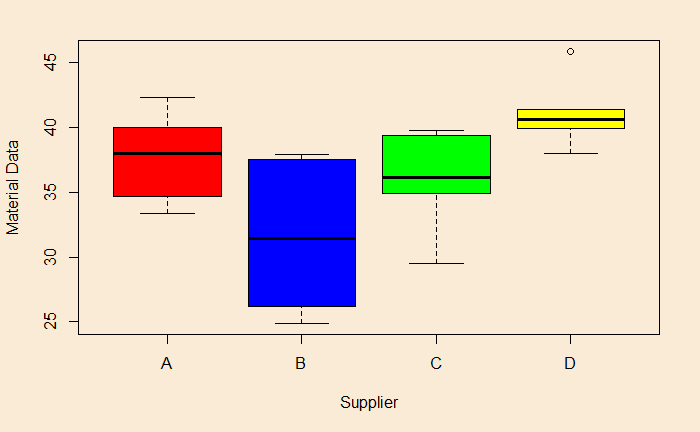
Here are the sampling results of a product from four suppliers, A, B, C and D (Data courtesy: https://statisticsbyjim.com/).
| A | B | C | D |
| 40 | 37.9 | 36 | 38 |
| 36.9 | 26.2 | 39.4 | 40.8 |
| 33.4 | 24.9 | 36.3 | 45.9 |
| 42.3 | 30.3 | 29.5 | 40.4 |
| 39.1 | 32.6 | 34.9 | 39.9 |
| 34.7 | 37.5 | 39.8 | 41.4 |
Hypotheses
N0 – All means are equal
NA – Not all means are equal
Input the data
PO_data <- read.csv("./Anova_Tukey.csv")
as_tibble(PO_data)
Leads to the output (first ten entries)
Material Strength
<chr>     <dbl>
B	  37.9
C	  36.0
D	  38.0
A	  40.0
A	  36.9
C	  39.4
A	  33.4
B	  26.2
B	  24.9
B	  30.3
Plot the data
par(bg = "antiquewhite")
colors = c("red","blue","green", "yellow")
boxplot(PO_data$Strength ~ factor(PO_data$Material), xlab = "Supplier", ylab = "Material Data", col = colors)
F-test for ANOVA
str.aov <- aov(Strength ~ factor(Material), data = PO_data)
summary(str.aov)
Output:
                 Df Sum Sq Mean Sq F value Pr(>F)
factor(Material)  3  281.7    93.9   6.018 0.0043 **
Residuals        20  312.1    15.6
---
Signif. codes:  0 ‘***’ 0.001 ‘**’ 0.01 ‘*’ 0.05 ‘.’ 0.1 ‘ ’ 1
Reject null hypothesis
We at least reject the null hypothesis because the p-value < 0.05 (the chosen significance level). The F-value is 6.018. Another way of coming the conclusions is to find out the critical F value for the degrees of freedoms, df1 = 3 and df2 = 20.
qf(0.05, 3,20, lower.tail=FALSE)
pf(6.018, 3, 20, lower.tail = FALSE)
Lead to
3.098391      # F-critical
0.004296141   # p-value for F = 6.018
Tukey’s test for multiple comparisons of means
TukeyHSD(str.aov)Tukey multiple comparisons of means
95% family-wise confidence level
Fit: aov(formula = Strength ~ factor(Material), data = PO_data)
$`factor(Material)`
diff lwr upr p adj
B-A -6.166667 -12.549922 0.2165887 0.0606073
C-A -1.750000 -8.133255 4.6332553 0.8681473
D-A 3.333333 -3.049922 9.7165887 0.4778932
C-B 4.416667 -1.966589 10.7999220 0.2449843
D-B 9.500000 3.116745 15.8832553 0.0024804
D-C 5.083333 -1.299922 11.4665887 0.1495298Interpreting pair-wise differences
You can see that the D-B difference, 9.5, is statistically significant at an adjusted p-value of 0.0022. And, as expected, the 95% confidence interval for D-B doesn’t include 0 (no difference between D and B).
By the way, the message, the difference between blue box and yellow, was already apparent had you paid attention to the box plots we made in the beginning.
Reference
Hypothesis Testing: An Intuitive Guide: Jim Frost

