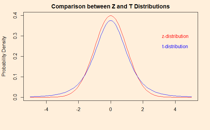
T-test closely resembles Z-test; both follow normal distributions. The t-test is relevant when the population standard deviation is unknown; instead, the sample standard deviation is used. After finding the test statistic, the t-test refers to the t-distribution for significance and p-values instead of the standard normal distribution.
![]()
T-distribution, unlike standard normal, is dependent on the sample size and is more spread for smaller values. A key term to remember is the degrees of freedom (df) = sample size – 1. A comparison between the two for a sample size of 5 (df = 4) is below.

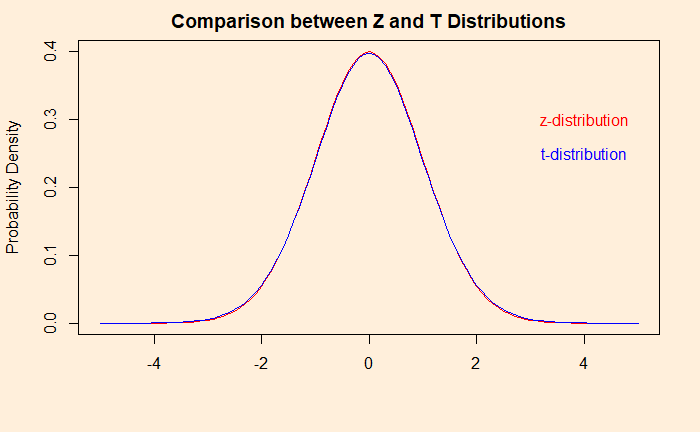
The difference soon disappears as the number of samples goes beyond a few. The plot below compares a sample size of 50.

Coffee Drinking
A researcher studies the coffee drinking habits of people and found that in her city, people drink 14 ml of extra coffee on Mondays (standard deviation of 8.5 ml). Can her results reject the existing average of 10 ml more on Mondays at a 5% significance level?
Let’s set up the null hypothesis: The average extra coffee consumed on Mondays is less than or equal to 10 ml. The alternative hypothesis is: The average extra coffee consumed on Mondays is more than 10 ml. No standard deviation is known for the population; therefore, we take sample standard deviation and t-statistic. t = (14-10)/(8.5 x sqrt(50)) = 3.327. The critical value for 0.05 significance level in a t-distribution with degrees of freedom (df) = 49 is 1.68 [qt(0.95,49) in R]. Since the t-statistic value (3.327) is greater than the t-critical value (1.68), we reject the null hypothesis. The p-value is 0.000838 [pt(3.327, 49, lower.tail = FALSE) in R].
The claim on weight reduction
T-tests can be used to validate claims of interventions by taking statistical differences of the same population between two conditions or time points. Company X claim success for its weight loss drug by showing the following data. You’ll test whether there’s any statistical evidence for the claim (at a 5% significance level).
| Before | After |
| 120 | 114 |
| 94 | 95 |
| 86 | 80 |
| 111 | 116 |
| 99 | 93 |
| 78 | 83 |
| 78 | 74 |
| 96 | 91 |
| 132 | 136 |
| 108 | 109 |
| 94 | 90 |
| 88 | 91 |
| 101 | 100 |
| 93 | 90 |
| 121 | 120 |
| 115 | 110 |
| 102 | 103 |
| 94 | 93 |
| 82 | 81 |
| 84 | 80 |
The steps are:
1) start with a null hypothesis: the average weight change (after medicine – before medicine) is zero.
2) calculate the weight difference by subtracting before from after (for 20 samples)
3) estimate the mean and standard deviation of the differences
4) population mean (for the null hypothesis) for weight difference is 0.
5) apply the formula for t-statistic
6) compare with critical t-value = -1.72 for 5% significance level
7) estimate the p-value
| Difference = After – Before |
| -6 |
| 1 |
| -6 |
| 5 |
| -6 |
| 5 |
| -4 |
| -5 |
| 4 |
| 1 |
| -4 |
| 3 |
| -1 |
| -3 |
| -1 |
| -5 |
| 1 |
| -1 |
| -1 |
| -4 |
The test shows no evidence to prove the effectiveness, and therefore, the null hypothesis is not rejected. The above treatment is called a paired t-test.
Business Analytics: U Dinesh Kumar

