It took quite some time and online help to get some of the R codes to generate the analysis of the last post. So let me share them with you.
The Data
The data was generated using the rnorm function, which is a random number generator using a normal distribution. The following lines of codes generate 10,000 random data points from a normal distribution, with an average of 67 and a standard deviation of 2.5, add them to a data frame, and plot the histogram.
theo_dat <- rnorm(10000, mean = 67, sd = 2.5)
height_data <- data.frame(Height = theo_dat)
par(bg = "antiquewhite")

hist(height_data$Height, main = "", xlab = "Height (inch)", ylab = "Frequency", col = c("grey", "grey", "grey", "grey", "grey", "grey", "grey","grey","brown","blue", "red", "green"), freq = TRUE, ylim = c(0,2000))
abline(h = 2000, lty = 2)
abline(h = 1500, lty = 2)
abline(h = 1000, lty = 2)
abline(h = 500, lty = 2)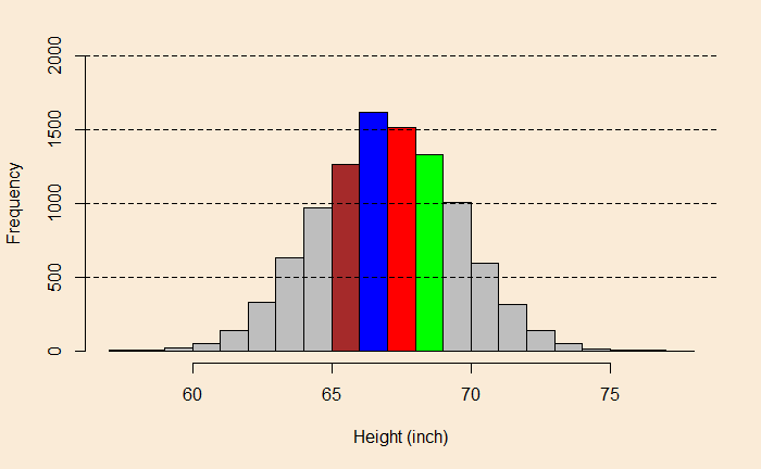
Horizontal lines are drawn to mark a few reference frequencies, and the option freq is turned ON (TRUE), which is the default. On the other hand, the density plot may be obtained by one of the two options: freq = FALSE or prob = TRUE.
par(bg = "antiquewhite")
hist(height_data$Height, main = "", xlab = "Height (inch)", ylab = "Density", col = c("grey", "grey", "grey", "grey", "grey", "grey", "grey","grey","brown","blue", "red", "green"), prob = TRUE, ylim = c(0,0.2))
abline(h = 0.2, lty = 2)
abline(h = 0.15, lty = 2)
abline(h = 0.1, lty = 2)
abline(h = 0.05, lty = 2)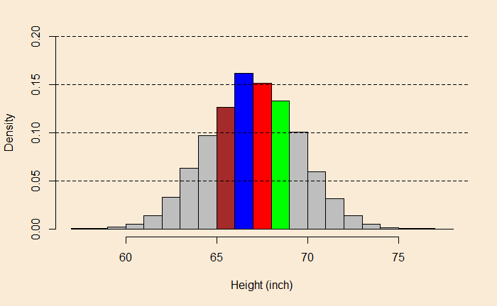
quantile function (stats library) can give quantiles at specified intervals, in our case, 5%.
quantile(height_data$Height, probs = seq(0,1,0.05))| 0% | 5% | 10% | 15% | 20% | 25% | 30% |
| 57.88 | 62.87 | 63.80 | 64.37 | 64.87 | 65.31 | 65.69 |
| 35% | 40% | 45% | 50% | 55% | 60% | 65% |
| 66.05697 | 66.37 | 66.69 | 66.98 | 67.29 | 67.62 | 67.97 |
| 70% | 75% | 80% | 85% | 90% | 95% | 100% |
| 68.31 | 69.10 | 69.56 | 68.70 | 70.15 | 71.06 | 77.55 |
A bunch of things are attempted below:
1) The spacing (breaks) of the histogram bins as per quantiles
2) Rainbow colours for the bins are given to the bins
3) Two X-axes are given one 2.5 units below another
vec <- rainbow(9)[1:10]
vic <- rev(vec)
mic <- c(vec,vic)
lab <- c("0%", "5%", "10%", "15%", "20%", "25%", "30%", "35%", "40%", "45%", "50%", "55%", "60%", "65%", "70%", "75%", "80%", "85%", "90%", "95%", "100%" )

par(bg = "antiquewhite")
hist(height_data$Height, breaks = quantile(height_data$Height, probs = seq(0,1,0.05)), col = mic, xaxt = "n", main = "", xlab = "", ylab = "Density")
axis(1, at = quantile(height_data$Height, probs = seq(0,1,0.05)) , labels=lab)
axis(1, at = quantile(height_data$Height, probs = seq(0,1,0.05)), line = 2.5)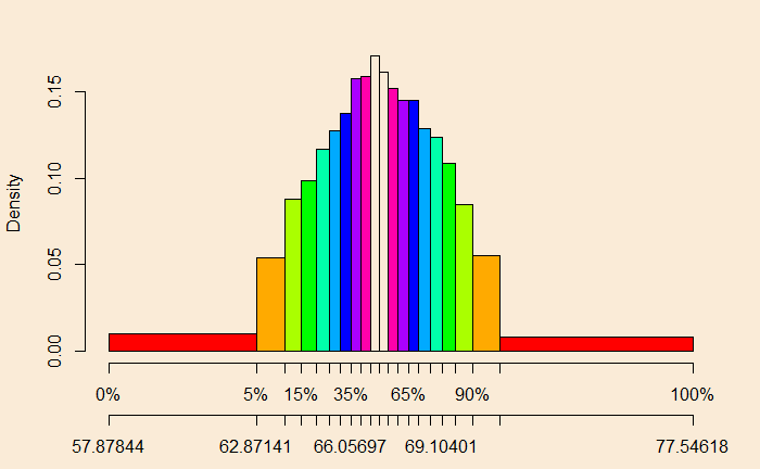
Note that the 10th bin (from the left came out with no colour as we selected 9 from the rainbow and 10 total array elements for the colour vector.
