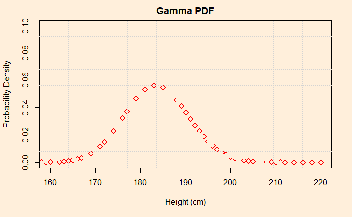
Yet another type of distribution – the Gamma distribution. It is an example of a continuous distribution. i.e. the data (or the random variable) can take any values within its range. Look at a variable like the weight of people. The values it can take vary, from its lower to upper bound, through infinite micrograms in between. Whereas the distributions we have seen so far (binomial and Poisson) had to restrict themselves to counts or tries of integer values.
As we did earlier for Poisson and Binomial, we plot the actual distribution of the random variable, probability density function and cumulative distribution function. Take a set of fictitious data from 200 Dutch adults for their heights.

The R function that creates random variables is rgamma, and takes two parameters, a and b – rgamma(a,b). One interesting thing about these two parameters is that the expectation (mean) of the distribution is (a/b), and the variance is (a/b2). Similarly, dgamma gives the PDF of the distribution.
plot(dgamma(220, 670.15, 3.65), xlim = c(160,220), ylim = c(0,.1), xlab="Height (cm)", ylab="Probability Density", col = "red", cex = 1, pch = 5, type = "p", bg=23, main="Gamma PDF")
grid(nx = 10, ny = 9)
Gamma distribution is used for modelling systems that lead to positive outcomes. The distribution is not symmetric. For the example we created, the mean comes out to be 670.15/3.65 = 183.6 and standard deviation = square root (670.15/3.652) = 7.1
There is a reason why I have introduced Gamma distribution immediately after the Poisson. That is for another post!
Height of Dutch Children from 1955 to 2009: Nature

