The Central Limit Theorem (CLT). It has intrigued me for a long time. The theorem concerns independent random variables, but it is not about the distribution of random variables. We know that a plot of independent random variables will be everywhere and should not possess any specific pattern. The central limit theorem is about the distribution of their sums. Remember this.
Let us take banks and defaulters to prove this point. Suppose a bank gives away 2000 loans. The bank knows that about 2.5% of the borrowers could default but does not know who those 50 individuals are! That means the defaulters are random. They are also independent. These are two highly debatable notions; once in a blue moon, these assumptions will prove to be the bank’s end. But we’ll deal with it later.
So, what is the distribution of losses to this bank due to defaults? Before that, why is it a distribution and not a fixed number, say, 50 times the loss per foreclosure? Or if the loss per foreclosure is 100,000 per loan, the total loss is 50 x 100,000 = 5 million. A fixed number. That is because a 2.5% default rate is a probability of defaulting, not a certainty. If it is a probability, the total loss to the bank is not a fixed amount but a set of random numbers.
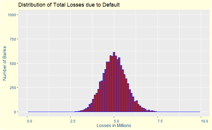
Let’s disburse 2000 loans to people and collect data from 10,000 banks worldwide! How do we do it? By Monte Carlo simulations. The outcome is given below as a plot.

This is the Central Limit Theorem! To put it in words, if we take a large number of samples from a population, and these samples are taken independently from each other, then the distribution of the sample sums (or the sample averages) follows a normal distribution.

