In the last post, we developed an MCMC algorithm for calculating the posterior probability distribution for the shark problem. We will do a few more things on it before closing out.
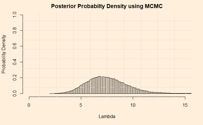
The first thing is to express the histogram in the form of Gamma distribution. We calculate the mean and variance of the data and apply the following formulae.
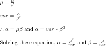
mean(lambda) = 7.45
var(lambda) = 3.72
sd(lambda) = 1.93
Now, check the post where we did the analytical solution for the hyperparameters of the posterior. Do they match?
Trace Plot
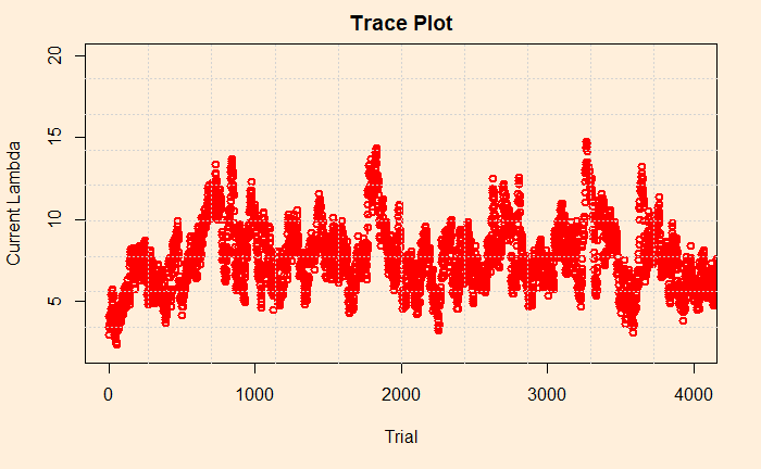
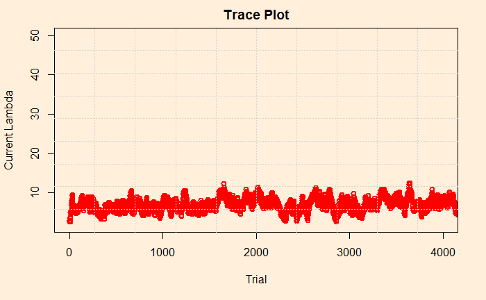
Trace plot is next. It is a line diagram connecting all the current lambdas against the trial number. The following plot gives the first 4000 (of the 100,000) trials we have performed.
Now we pick the first 40 to zoom in on the values.
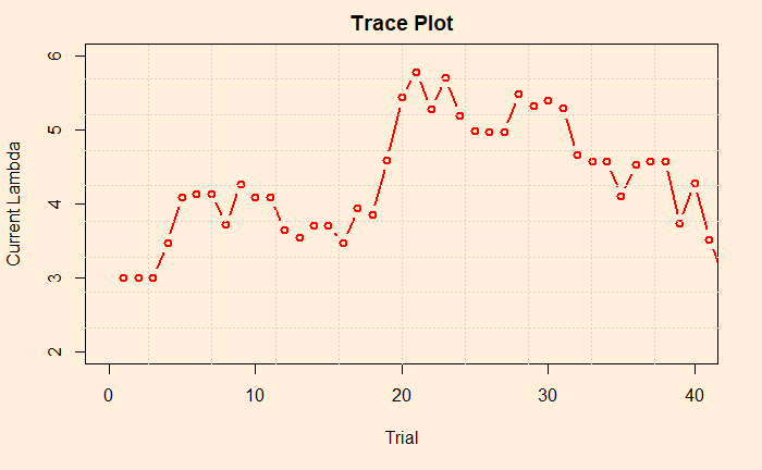
By looking at the plot, you may recognise the concept known as the acceptance rate. It is the percentage of instances where the current lambda got rejected in favour of the proposed. In the figure, there are approximately three in four times the points jumped (up or down) to a new value. There are recommendations to keep the acceptance rates between 25 – 50% as a good practice. You can tune the rate by varying the standard deviation of the normal distribution (step 3 of the MCMC scheme).
Impact of starting lambda
Finally, we look into the sensitivity of prior. We had arbitrarily chosen 3 in the previous exercise. Here is the trace plot once again.
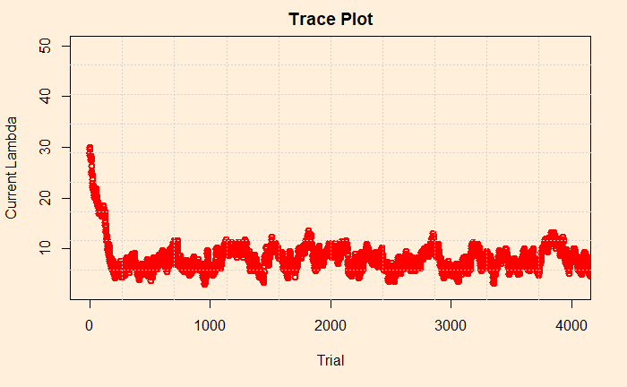
What about changing it to 30? We could see that the distribution remained the same (after 100,000 iterations). Let’s check the trace plot. You will notice that it was higher, to begin with, but came down in a few trials.
Reference
Bayesian Statistics for Beginners: a step-by-step approach, Donovan and Mickey

