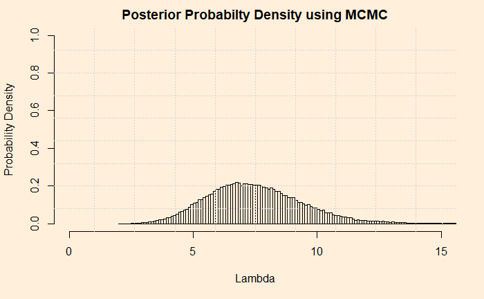
So far, we have created an analytical solution to the Poisson-Gamma conjugate problem. Now, it is time for the next step: a numerical solution using the Markov Chain Monte Carlo (MCMC) method. The plan is to go stepwise and develop R codes side by side.
Markov Chain Monte Carlo
We write the Bayes’ theorem in the following form,
![]()
Step 0: The Objective
The objective of the exercise is to calculate the probability density of the posterior (updated hypothesis) given the (new) data at hand. As we did previously, we will need to use the hyperparameters alpha and beta.
data_new <- 10
alpha <- 5
beta <- 1
Step 1: Guess a Lambda
You start with one value for the posterior distribution (of lambda). It can be anything reasonable; I just took 3. It is an arbitrary selection. We can think of changing to something else later.
current_lambda <- 3Step 2: Calculate the Likelihood, prior and posterior
Use the guess value of lambda and calculate the likelihood using Poisson PMF. In other words, get the chance of occurrence of a rare independent event 5 times in a year if the lambda was 3.
liklely_current <- dpois(data_new,current_lambda) Calculate the prior probability density associated with the lambda (value of the posterior) for the given hyperparameters, alpha and beta. Sorry, I forgot: use Gamma PDF.
prior_current <- dgamma(current_lambda, alpha, beta)The next one is obvious, use the calculated values of prior and likelihood and calculate the probability density of the posterior using the new form of the Bayes’ equation.
post_current <- liklely_cur*prior_currentStep 3: Draw a Random Lambda
The second value of lambda is selected at random from a symmetrical distribution that is centred at the current value of lambda. We will use a normal distribution for that. We’ll call the new value, the proposed lambda. I used the absolute value because the new value can pick negative once in a while and lead the program to terminate.
mu_rand <- current_lambda
sd_rand <- 0.5
proposed_lambda <- abs(rnorm(1, mu_rand, sd_rand))
Step 4: Step 2 Reloaded
We will calculate the posterior PDF the same way we did in step 2.
liklely_proposed <- dpois(data_new,proposed_lambda)
prior_proposed  <- dgamma(proposed_lambda,  alpha, beta)
post_proposed <- liklely_proposed*prior_proposed
Step 5: Calculate the Probability of Moving
Now you have two posterior values, post_current and post_proposed. We go to throw one out. How do we make that decision? Here comes the famous Metropolis algorithm to the rescue. It specifies to pick the smaller of the two between 1 and the ratio of the two posteriors. The resulting value is the probability of moving to the new lambda.
prob_move <- min(post_proposed/post_current, 1)
Step 6: New Lambda or the Old
The verdict (to move or not) is not out yet! Now, draw a random number from a uniform distribution and compare it. If your number is higher than the random number, move to the new lambda, and if not, stay with the old lambda.
rand_uniform <- runif(1)
if(prob_move > rand_uniform) {
  current_lambda <- proposed_lambda
}
Step 7: Repeat the Process
You have done one iteration, and you have a lambda (switch to new or retain the old). Now, you go back to step 2 and repeat all steps. Thousands of times until you meet the set iteration number, for example, one hundred thousand!
n_iter <- 100000
for (x in 1:n_iter) {
}
Step 8: Collect All the Accepted Values
Ask the question: what is the probability density distribution of the posterior? It is the normalised frequency of lambda values. Note that I just omitted the condition, “given the data”, to keep it simple, but don’t forget, it is always the conditional probability. You may get the histogram from the frequency data using the attribute “freq = FALSE”. See below
lambda[x] <- current_lambda
hist(lambda, freq = FALSE)
Putting All Together
data_new  <- 10
alpha <- 5# shape
beta <- 1  # rate

current_lambda  <- 3

n_iter <- 100000  # number of iterations
lambda <- rep(0, n_iter) # initialise a vector with zeros
x_val <- rep(0, n_iter)  # initialise a vector with zeros

for (x in 1:n_iter) {

lambda[x] <- current_lambda
x_val[x] <- x
liklely_current <- dpois(data_new,current_lambda)
prior_current  <- dgamma(current_lambda, alpha, beta)
post_current <- liklely_current*prior_current

mu_rand <- current_lambda
sd_rand <- 0.5
proposed_lambda <- abs(rnorm(1, mu_rand, sd_rand)) # negative values, if they occur, will mess up the calculation

liklely_proposed <- dpois(data_new,proposed_lambda)
prior_proposed  <- dgamma(proposed_lambda,  alpha, beta)
post_proposed <- liklely_proposed*prior_proposed

prob_move <- min(post_proposed/post_current, 1)

rand_uniform <- runif(1)# generates 1 uniform random number between 0 and 1
if(prob_move > rand_uniform) {
  current_lambda <- proposed_lambda
}


}

xx <- seq(0,20, 0.1)
par(bg = "antiquewhite1")
hist(lambda, breaks = 200, freq = FALSE, xlim = c(0,15), ylim = c(0,1), main = "Posterior and Prior", xlab="Number", ylab="Probability Density")

grid(nx = 10, ny = 9)
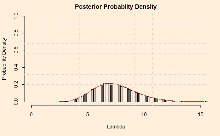
But how do you know it worked? Let’s compare it with the analytical solution from the previous post. The red line represents the analytical solution.

Reference
Bayesian Statistics for Beginners: a step-by-step approach, Donovan and Mickey

