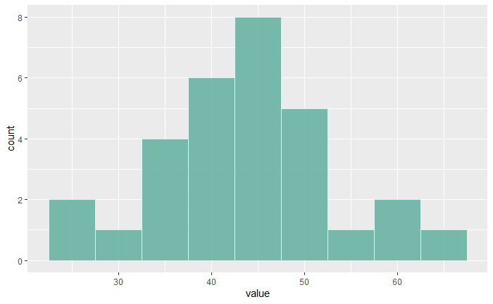
In the last post, we used a non-parametric hypothesis test, the Wilcoxon Signed Rank test. The p-value showed that the evidence was not sufficient to reject the null hypothesis. However, the histogram suggests that the data was reasonably a normal distribution.

Shapiro-Wilk test is a formal way of testing whether the data follows a normal distribution or not. The test has a null hypothesis that the sample comes from a normally distributed population. The test statistics, W has the following formula:
![]()
We can apply the Shapiro-Wilk test to our data using the following R code:
diab <- c(35.5, 44.5, 39.8, 33.3, 51.4, 51.3, 30.5, 48.9, 42.1, 40.3, 46.8, 38.0, 40.1, 36.8, 39.3, 65.4, 42.6, 42.8, 59.8, 52.4, 26.2, 60.9, 45.6, 27.1, 47.3, 36.6, 55.6, 45.1, 52.2, 43.5)

shapiro.test(diab)
Shapiro-Wilk normality test
data: diab
W = 0.98494, p-value = 0.9361
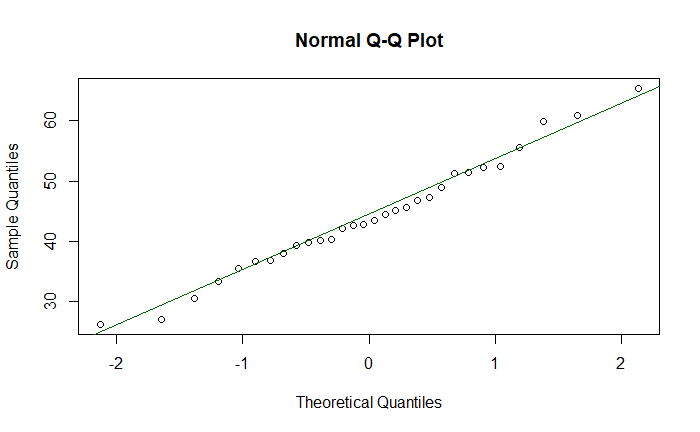
The p-value is quite high, and the null hypothesis is not rejected. The same conclusion may be obtained by doing a q-q plot as follows.
qqnorm(diab)
qqline(diab, col = "darkgreen")

