We have been hearing about hypothesis testing a lot. But what is that in reality? We will resolve it systematically by working with samplings from a large – computer-generated – population.
What is hypothesis testing?
It is a tool to express something about a population from its small subset, known as a sample. If one measures the heights of 20 men in the city centre, does something with the data and makes a claim about men in the city, it qualifies as a hypothesis. Imagine if it was a cunning journalist who measured the heights (mean = 163 cm and standard deviation = 20 cm) and reported that the people in the city were seriously undersized (the national average is 170), a claim the mayor vehemently disputes.
So, we need someone to perform a hypothesis test assessing two mutually exclusive arguments about the city’s population and tell which one has support from the data. The mayor says the average is 170, and the journalist says it’s not.
The arguments
Null hypothesis: The population mean equals the national average (170 cm).
Alternate hypothesis: The population mean does not equal the national average (170 cm).
Build the population
The city has 100,000 men, and their height data is available to an alien. The average is, indeed, 170 cm. And do you know how she got that information? By running the following R code:
n_pop <- 100000
pop <- rnorm(n_pop, mean = 170, sd = 17.5)
Don’t you believe it? Here they are:

The journalist took a sample of 30 from it. So the statistician’s job is to verify if his number (sample mean of 163 cm at sample standard deviation of 20 cm) is possible from this population.
Test statistic
Calculating a suitable test statistic is the first step. A statistic is a measure that is applied to a sample, e.g., sample mean. If the same is done to a population, it is called a parameter. So population parameters and sample statistics. For the given task, we chose a t-test statistic by smartly combining the mean and standard deviation of the sample into a single term in the following fashion:
![]()
X bar is the sample mean
mu0 is the null value
s is the sample standard deviation and
n is the number of individuals in the sample
For the present case, it is:
![]()
Why is that useful?
To understand the purpose of the t-test statistics, we go back to the alien. It collected 10,000 samples, 30 data points at a time, from the population, and here is how it was obtained.
itr <- 10000

t_val <- replicate(itr, {
n_sam <- 30
sam <- sample(pop, n_sam, replace = FALSE)
t_stat <- (mean(sam) - 170)/(sd(sam) / sqrt(n_sam))
})
You can already suspect that our t-value of -1.92, obtained from an average of 163 cm, is not improbable for a population average of 170 cm. In other words, getting a sample mean of 163 is “natural” within the scatter (distribution) of heights. If you are not sure how t-values change, try substituting 162, and you get -2.2 (higher magnitude, further away from the middle).
t-distribution
Luckily, there has been a standard distribution that resembles the above histogram created from the subsamples. As per wiki, the t-distribution was first derived in 1876 by Helmert and Lüroth. It is of the following form.
![]()
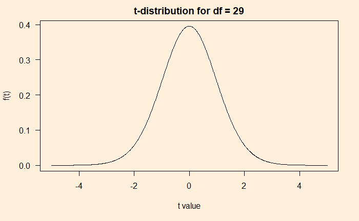
The beauty of this function is that it has only one parameter, df (number of data points – 1). The plot of the function for df = 29 is below.
x_t <- seq(- 5, 5, by = 0.01)
df <- 29

y_t <- gamma((df+1)/2)(1+(x_t^2)/df)^(-(df+1)/2)/(sqrt(df*3.14)*gamma(df/2))

plot(x_t, y_t, type = "l", main = "t-distribution for df = 29", xlab = "t value", ylab = "f(t)")
Combining distributions
Before going forward with inferences, let’s compare the sampling distribution (from 10000 samples as carried out by the alien) with the t-distribution we just evaluated.

Pretty decent fitting! Although, in reality, we never get a chance to produce the sampling distribution (the histogram), we do not need that anymore as we are convinced that the t-distribution will work instead.
Verdict of the test
The t-statistic derived from the sample, -1.92, is within the distribution if the average height of 170 cm is valid for the population. But by how much? One way to specify an outlier is by agreeing on a significance value; the statistician’s favourite is 95%. It means if the t value of the sample (the value of the x-axis) is in such a way that it is part of 95% of the distribution, then the sample mean that produced the t-value is valid. In the following figure, the 95% coverage is shaded, and our statistic is denoted as a red dot. In summary: a value of 163 cm is perfectly reasonable in the universe of 170!

Based on this, the collected data is not sufficient to dislodge the null hypothesis – a temporary respite for the mayor. Interestingly, the data can never prove he was right – it only says there is insufficient ground to reject his position.

