Regression: The OLS Way

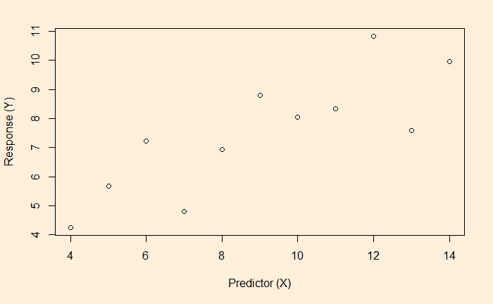
OLS is the short form for ordinary least squares and is a linear regression method. The process is also known as curve fitting informally. The objective is to find the relationship between the dependent (the y) and independent (the x) variables; one eventually gets (to predict) the variation of y from the variation of x. In case you forgot, here is the scatter plot of the data.

^{x = (10, 8, 13, 9.0, 11.0, 14.0, 6.0, 4.0, 12.0, 7.0, 5.0); y = (8.04, 6.95, 7.58, 8.81, 8.33, 9.96, 7.24, 4.26, 10.84, 4.82, 5.68)}

We start with the equation of a line; because we fit a line (linear regression).

$y = a x + b$

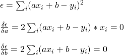
Now, the equation for the residuals, i.e. deviations of actual y from the model y.

$\\ y - y_i = a x_i + b - y_i$

As you’ve already guessed, square the residuals, sum them and find the values of the constants, a and b, that minimise the sum.

$\\ \epsilon = \sum_i (a x_i + b - y_i)^2 \\ \\ \frac{\delta\epsilon}{\delta a} = 2 \sum_i (a x_i + b - y_i) * x_i = 0 \\ \\ \frac{\delta\epsilon}{\delta b} = 2 \sum_i (a x_i + b - y_i) = 0$

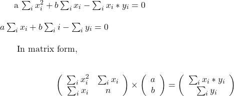
The above equations lead to two sets of linear equations that need to be solved.

$\\ a \sum_i x_i^2 + b \sum_i x_i - \sum_i x_i *y_i = 0 \\ \\ a \sum_i x_i + b \sum_i i - \sum_i y_i = 0 \\ \text{ In matrix form, } \\ \[ \left( \begin{array}{cc} \sum_i x_i^2 & \sum_i x_i \\ \sum_i x_i & n \end{array} \right) \times \[ \left( \begin{array}{c} a \\ b \end{array} \right) = \[ \left( \begin{array}{cc} \sum_i x_i*y_i \\ \sum_i y_i \end{array} \right)$

We solve this equation for a and b using the following r code


Q1 <- data.frame("x" = c(10, 8, 13, 9.0, 11.0, 14.0, 6.0, 4.0, 12.0, 7.0, 5.0), "y" = c(8.04, 6.95, 7.58, 8.81, 8.33, 9.96, 7.24, 4.26, 10.84, 4.82, 5.68))

x_i_2  <-  sum(Q1$x*Q1$x)
x_i  <-  sum(Q1$x)
nn <- nrow(Q1)

x_i_y_i <- sum(Q1$x*Q1$y)
y_i <- sum(Q1$y)


X <- matrix(c(x_i_2, x_i, x_i, nn), 2, 2, byrow=TRUE)
y <- c(x_i_y_i,y_i)

solve(X, y)

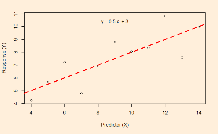
We get a = 0.5 (slope) and b = 3.0 (intercept). Now use the shortcut R code (“lm“) to verify

mm <- lm(Q1$y ~ Q1$x)

summary(mm)

Call:
lm(formula = Q1$y ~ Q1$x)

Residuals:
     Min       1Q   Median       3Q      Max 
-1.92127 -0.45577 -0.04136  0.70941  1.83882 

Coefficients:
            Estimate Std. Error t value Pr(>|t|)   
(Intercept)   3.0001     1.1247   2.667  0.02573 * 
Q1$x          0.5001     0.1179   4.241  0.00217 **
---
Signif. codes:  0 ‘***’ 0.001 ‘**’ 0.01 ‘*’ 0.05 ‘.’ 0.1 ‘ ’ 1

Residual standard error: 1.237 on 9 degrees of freedom
Multiple R-squared:  0.6665,	Adjusted R-squared:  0.6295 
F-statistic: 17.99 on 1 and 9 DF,  p-value: 0.00217

The original scatter plot with the model line included

Related Posts