Regression – Stock Index Performance

We will continue the regression, and this time, we’ll apply it to stock market performance. Below is the weighted average performance of the top 50 stocks listed in India’s National Stock Exchange, known as the NIFTY 50 benchmark index.

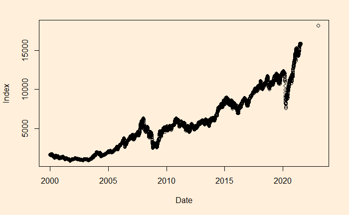
We want to perform regression of the data using a power law approximation of the following form.

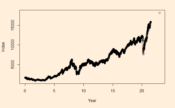
There is a reason to write the function in the above format, as the constant r value can represent the underlying stocks’ average CAGR (compound annual growth rate). Before we proceed, let’s convert the x-axis to time (in years) using the following R code.

Nif_data$Year <- time_length(difftime(Nif_data$Date, Nif_data$Date[1]), "years") 

The function “time_length()” comes from the “lubridate” package.

We’ll transfer the function to linear form and do an OLS fit.

The slope of this has to be ln(1+r) and intercept be ln(index₀)

Nif_data$ln <- log(Nif_data$Index)
plot(Nif_data$Year, Nif_data$ln, xlab = "Year", ylab = "Ln(Index)")
abline(lm(Nif_data$ln ~ Nif_data$Year), col = "red", lty = 2, lwd = 3)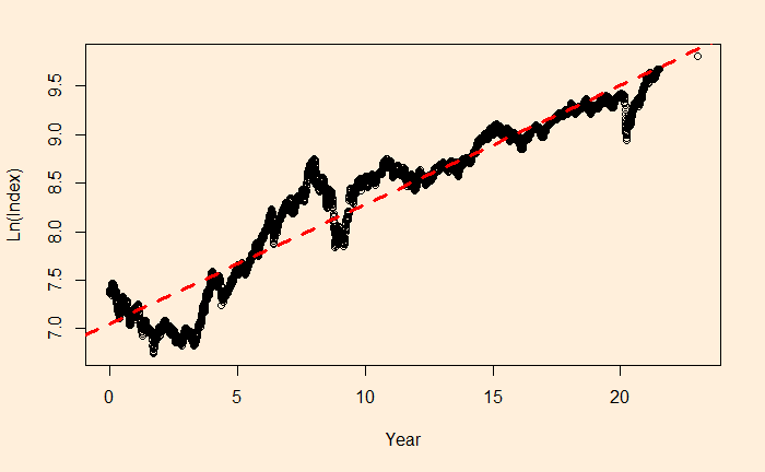

fit <- lm(ln ~ Year, data=Nif_data)
summary(fit)

Call:
lm(formula = ln ~ Year, data = Nif_data)

Residuals:
     Min       1Q   Median       3Q      Max 
-0.62561 -0.11342 -0.02233  0.15665  0.71261 

Coefficients:
             Estimate Std. Error t value Pr(>|t|)    
(Intercept) 7.0476743  0.0063781  1105.0   <2e-16 ***
Year        0.1230505  0.0005146   239.1   <2e-16 ***
---
Signif. codes:  0 ‘***’ 0.001 ‘**’ 0.01 ‘*’ 0.05 ‘.’ 0.1 ‘ ’ 1

Residual standard error: 0.2341 on 5352 degrees of freedom
Multiple R-squared:  0.9144,	Adjusted R-squared:  0.9144 
F-statistic: 5.718e+04 on 1 and 5352 DF,  p-value: < 2.2e-16

Converting them back, Index₀ = exp(7.0476743) = 1150.181 and r = exp(0.1230505) – 1 = 0.1309415 or 13.09%.

xx <- seq(0,30)
plot(Nif_data$Year, Nif_data$Index, xlim = c(0,30), ylim = c(0,19000), xlab = "Year", ylab = "Index")
lines(xx, exp(fit$coefficients[1])exp(fit$coefficients[2]xx), col = "red", lty = 2, lwd = 3)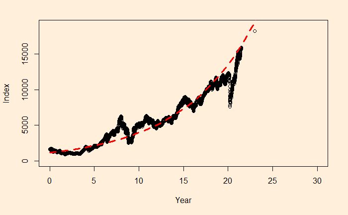

Obviously, this is an approximate estimation of the CAGR. If you want an accurate value, use the direct formula (Index_fin/Index_ini)^(1/Year) – 1

(Nif_data$Index[5354]/Nif_data$Index[1])^(1/Nif_data$Year[5354]) - 1

which gives 0.1117364 or 11.17%

The main reason for such a discrepancy (a 2% difference is a big deal for long-term compounding) between the two estimates is the less accurate intercept of regression. The actual intercept or index₀ is 1592.20, which is so different from the estimated value of 1150.181.