With all its simplicity, portfolio theory still describes the value in grouping securities, preferably ones uncorrelated with each other, for more predictable returns. The statistical parameters, mean and standard deviation, representing the expected return and risk, respectively, also suggest an underlying probability distribution. Despite all criticism around the usage or normal distribution (symmetric bell curve), we still utilise it to explain the portfolio concept.
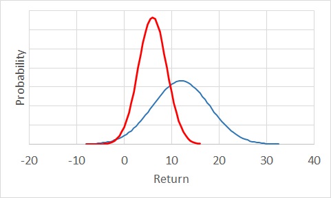
In the previous post, we saw two stocks, 1 and 2, with two different expected returns (12 and 6) and risks (6 and 3). If the overall returns followed a normal distribution, they would have appeared like in the following plot.

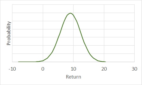
Here, the blue curve represents the one with a higher expected return and higher volatility. The red one is more conservative. The combined set (1:1) for a correlation coefficient of 0 (uncorrelated) behaves in the following way.

The advantage of using a standard distribution (normal, in this case) is that it enables us to estimate various probabilities. E.g., the chance of ending up with a zero return and below for the blue curve (aggressive one) is 2.3%, which is similar to what the conservative (red) can give. On the other hand, for the joint distribution (green curve), it is just 0.4%.

