Normal – Normal Continued

We will do a few sensitivities and see how the posterior distribution modifies. Let’s define the variables before we start.

$\\ \mu = \text {variable}; \sigma = 2 \text { (hypothesis)} \\ \\ \mu_0 = 15; \sigma_0 = 4 \text { (prior)} \\ \\ x = 9 \text{ (data)}$

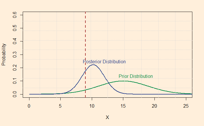
The plots of the distributions are

Imagine you collected four more data, and interestingly they are all the same, 9! You have five data points now, although the average remains the same (9) as the previous case.

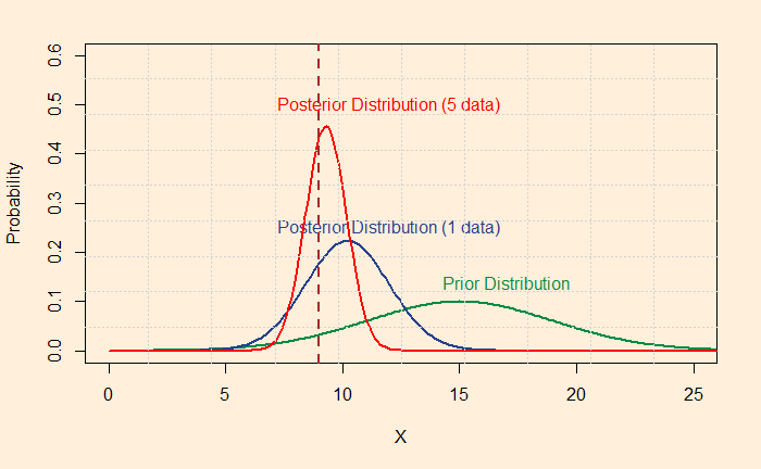
Note that the vertical dotted line represents the data (or the average of the data).

The relations used in the calculations of the posteriors are:

$\\ \mu_{posterior} = \frac{\tau_0 \mu_0 + \tau \Sigma_{i=1}^{n} x_i}{\tau_0 + n\tau} \\ \\ \tau_{posterior} = \tau_0 + n\tau \\ \\ \sigma_{posterior} = \sqrt{\frac{1}{\tau_{posterior} }}$

Related Posts