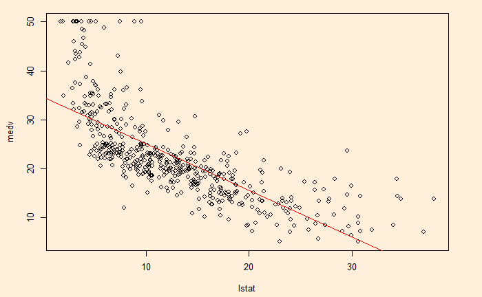
If you recall one of the previous posts relating ‘lstat’ with ‘medev’, we noticed the apparent curvature of the relationship. And how slightly awkward the fit-line on top of the scatter plot was.

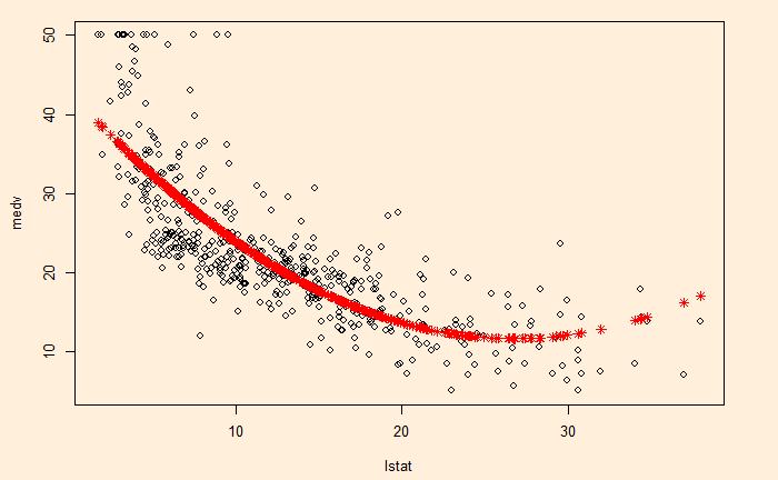
This seeming ‘non-linearity’ prompts us to extend the linear model to non-linear. We use a quadratic term by squaring the predictor (‘lstat’). We must use the identity function to do this.
fit5 <- lm(medv ~ lstat + I(lstat^2), Boston)The results are presented below:
Call:
lm(formula = medv ~ lstat + I(lstat^2), data = Boston)

Residuals:
     Min       1Q   Median       3Q      Max
-15.2834  -3.8313  -0.5295   2.3095  25.4148

Coefficients:
             Estimate Std. Error t value Pr(>|t|)
(Intercept) 42.862007   0.872084   49.15   <2e-16 ***
lstat       -2.332821   0.123803  -18.84   <2e-16 ***
I(lstat^2)   0.043547   0.003745   11.63   <2e-16 ***
---
Signif. codes:  0 ‘***’ 0.001 ‘**’ 0.01 ‘*’ 0.05 ‘.’ 0.1 ‘ ’ 1

Residual standard error: 5.524 on 503 degrees of freedom
Multiple R-squared:  0.6407,	Adjusted R-squared:  0.6393
F-statistic: 448.5 on 2 and 503 DF,  p-value: < 2.2e-16
Now, let’s compare the fit results.
plot(medv~lstat, Boston)
points(Boston$lstat, fitted(fit5), col = "red", pch = 8)

