We have seen linear regression before as a simple method in supervised learning. It is of two types – simple and multiple linear regressions. In simple, we write the dependent variable (also known as the quantitative response) Y as a function of the independent variable (predictor) X.

Beta0 and beta1 are the model coefficients or parameters. You may realise they are the intercept and slope of a line, respectively. An example of a simple linear regression is a function predicting a person’s weight (response) from her height (single predictor).
Multiple linear regression
Here, we have more than one predictor. The general form for p predictors is:
![]()
We use the Boston data set from the library ISLR2 for the R exercise. The library contains ‘medv’ (median house value) for 506 census tracts in Boston. We will predict ‘medv’ using 12 predictors such as ‘rm’ (average number of rooms per house), ‘age’ (proportion of owner-occupied units built before 1940), and ‘lstat’ (per cent of households with low socioeconomic status).
First, we do the simple linear regression with one predictor, ‘lstat’.
fit1 <- lm(medv~lstat, Boston)
summary(fit1)
Call:
lm(formula = medv ~ lstat, data = Boston)
Residuals:
Min 1Q Median 3Q Max
-15.168 -3.990 -1.318 2.034 24.500
Coefficients:
Estimate Std. Error t value Pr(>|t|)
(Intercept) 34.55384 0.56263 61.41 <2e-16 ***
lstat -0.95005 0.03873 -24.53 <2e-16 ***
---
Signif. codes: 0 ‘***’ 0.001 ‘**’ 0.01 ‘*’ 0.05 ‘.’ 0.1 ‘ ’ 1
Residual standard error: 6.216 on 504 degrees of freedom
Multiple R-squared: 0.5441, Adjusted R-squared: 0.5432
F-statistic: 601.6 on 1 and 504 DF, p-value: < 2.2e-16
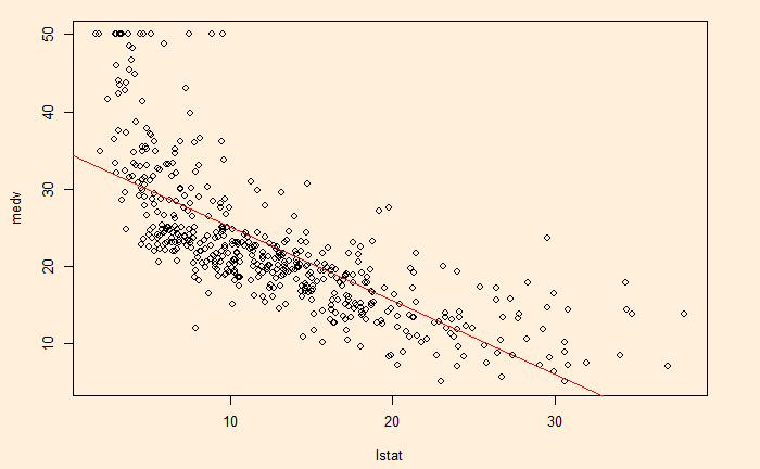
Here is the plot with points representing the data and the line representing the model fit.
fit1 <- lm(medv~lstat, Boston)
plot(medv~lstat, Boston)
abline(fit1, col="red")
We will add another predictor, age, to the regression table.
fit2 <- lm(medv~lstat+age, Boston)
summary(fit2)
Call:
lm(formula = medv ~ lstat + age, data = Boston)
Residuals:
Min 1Q Median 3Q Max
-15.981 -3.978 -1.283 1.968 23.158
Coefficients:
Estimate Std. Error t value Pr(>|t|)
(Intercept) 33.22276 0.73085 45.458 < 2e-16 ***
lstat -1.03207 0.04819 -21.416 < 2e-16 ***
age 0.03454 0.01223 2.826 0.00491 **
---
Signif. codes: 0 ‘***’ 0.001 ‘**’ 0.01 ‘*’ 0.05 ‘.’ 0.1 ‘ ’ 1
Residual standard error: 6.173 on 503 degrees of freedom
Multiple R-squared: 0.5513, Adjusted R-squared: 0.5495
F-statistic: 309 on 2 and 503 DF, p-value: < 2.2e-16beta_0 is 33.22, beta_1 is -1.03 and beta_2 is 0.034. All three are significant, as evidenced by their low p-values (Pr(>|t|)). We will add more variables next.
An introduction to Statistical Learning: James, Witten, Hastie, Tibshirani, Taylor

