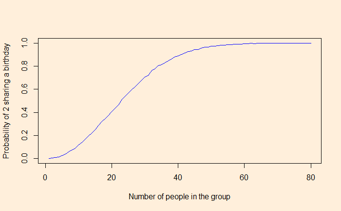
We have seen the birthday problem earlier. A group of 23 has a 50% chance that two members will share a birthday.
The R code that scans the probability of two people sharing a birthday against the number of people in the group is given by:
birth_day <- function(people, iterations, probs){
  birth <- replicate(iterations, {
    days <- sample(1:366, people, replace = TRUE, prob = probs)
    duplicated(days) %>% max()
  })
  mean(birth)
}

itr <- 80
b_day <- rep(0, itr)

for (i in 1:itr) {
   b_day[i] <- birth_day(i, 10000, rep(1/366, 366))
}
You don’t really need to write such lengthy codes, as R has a built-in function, ‘pbirthday’, that calculates the birthday probability.
for (i in 1:80) {
  b_day[i] <- pbirthday(i, classes = 366, coincident = 2)
}
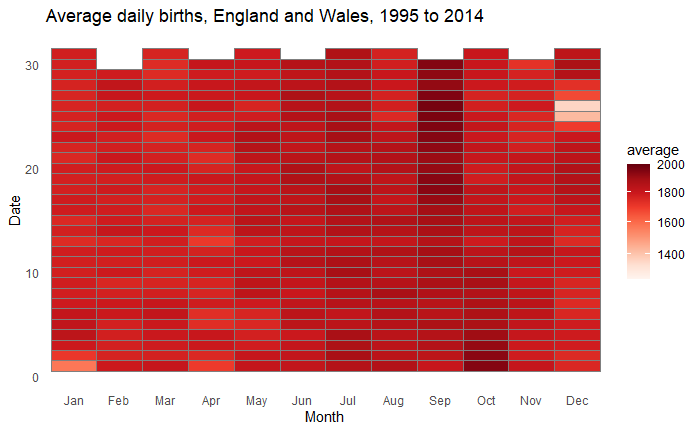
The two assumptions used in this work are that birthdays are independent and equally likely. However, these are not guaranteed to be true in real life. Here is an example of how births are distributed: the average daily births in England and Wales from 1995 to 2014.

Some months, such as July, September and October, are more popular than others for giving birth. But does it make the probabilities of the birthday problem different from the theory? We will see that next.
Reference
How popular is your birthday?: ONS

