Markov Chains – The Stable End Distribution

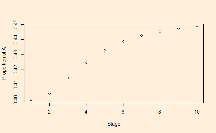
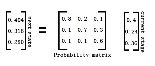
We have seen that the initial distribution of counts (or the proportion) reaches a stable state after a few generations.

In other words, the (n+1)^th and the n^th give the same result for the same given initial distribution and the probability matrix.

Let’s work out for n = 10. X₁₀ = P¹⁰ X₀

pM <- matrix(c(0.8, 0.1, 0.1, 0.2, 0.7, 0.1, 0.1, 0.3, 0.6), nrow = 3)
stage0 <- c(0.4, 0.24, 0.36)
stage10 <- pM%*%pM%*%pM%*%pM%*%pM%*%pM%*%pM%*%pM%*%pM%*%pM%*%stage0 
stage10

       [,1]
[1,] 0.45
[2,] 0.35
[3,] 0.20

And then for n = 11. X₁₁ = P¹¹ X₀

pM <- matrix(c(0.8, 0.1, 0.1, 0.2, 0.7, 0.1, 0.1, 0.3, 0.6), nrow = 3)
stage0 <- c(0.4, 0.24, 0.36)
stage11 <-pM%*%pM%*%pM%*%pM%*%pM%*%pM%*%pM%*%pM%*%pM%*%pM%*%pM%*%stage0  
stage11

     [,1]
[1,] 0.45
[2,] 0.35
[3,] 0.20

It would be interesting to see how the probability matrix is transformed as the number of stages progresses. Here is the original matrix (P), followed by (P¹⁰).

0.8  0.2  0.1
0.1  0.7  0.3
0.1  0.1  0.6       

0.45 0.45 0.45
0.35 0.35 0.35
0.20 0.20 0.20

Elements in each raw are similar in magnitude, which suggests why the end result after multiplying it with the original proportion is the same after each stage.

Another interesting fact is how X_n changes with the initial proportion, X₀. We use the following X₀ values. Note that the sum of the proportions must add to 1.

stagen %*% c(0.4, 0.24, 0.36)
stagen %*% c(0.3, 0.4, 0.3)
stagen %*% c(0.1, 0.1, 0.8)
stagen %*% c(0.1, 0.8, 0.1)

There is no prize for guessing – they all lead to the same X_n value!

0.45
0.35
0.20