Logistic Regression and Accuracy Paradox

The next step is to assign a cut-off probability value for decision-making. Based on that, the decision-maker will classify the observation as either class 1 or 0. If P_c is that cut-off value, the following condition occurs.

$Y_i = \begin{cases} 0, & \text{if } P(Y_i = 1) < P_c \\ 1, & \text{if } P(Y_i = 1) \ge P_c \end{cases}$

The following classification table is obtained if the cut-off value is 0.5.

$\\ ln(\frac{P(Y = 1)}{1 - P(Y = 1)}) = \beta_0 + \beta_1 X_i \text{ OR} \\ \\ P(Y = 1) = \frac{e^{\beta_0 + \beta_1 X_i}}{1 + e^{\beta_0 + \beta_1 X_i}} \\ \\ P(Y = 1) = \frac{e^{15.2968142 - 0.2360207 X_i}}{1 + e^{15.2968142 - 0.2360207 X_i}}$

Launch T (F)	Actual Damage	Prediction (P_c = 0.5)
66	0	0
70	1	0
69	0	0
80	0	0
68	0	0
67	0	0
72	0	0
73	0	0
70	0	0
57	1	1
63	1	1
70	1	0
78	0	0
67	0	0
53	1	1
67	0	0
75	0	0
70	0	0
81	0	0
76	0	0
79	0	0
75	1	0
76	0	0
58	1	1

The accuracy of the prediction may be obtained by counting the actual and predicted values or by using the function, ‘confusionMatrix’ of the ‘caret’ library.

True Positive (TP) = Damage = 1 & Prediction = 1
False Negative (FN) = Damage = 1 & Prediction = 0
False Positive (FP) = Damage = 0 & Prediction = 1
True Negative (TN) = Damage = 0 & Prediction = 0

Sensitivity = TP / (TP + FN) =  0.57 (57%)
Specificity  = TN / (TN + FP) = 1 (100%)
overall accuracy = (TP + TN) / (TP + TN + FN + FP) = 0.875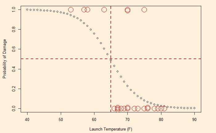

Although the overall accuracy is at an impressive 87.5%, the true positive rate or the failure estimation rate is pretty average (57%). Considering the significance of the decision, one way to deal with it is to increase the sensitivity by reducing the cut-off probability to 0.2. That leads to the following.

Sensitivity = TP / (TP + FN) =  0.857 (85.7%)
Specificity  = TN / (TN + FP) = 0.53 (53%)
overall accuracy = (TP + TN) / (TP + TN + FN + FP) = 0.625

Accuracy Paradox

As you can see, the sensitivity of the second case, the lower cut-off value, is higher, but the overall accuracy of the prediction is poorer. And this is a key step of decision making – choosing higher accuracy of predicting failures (positive values) over the overall classification accuracy.

Accuracy Paradox

Related Posts