Regression is a tool that enables us to find the relationship between two variables. The most commonly used one among them is linear regression, where we find the dependant variation (y) as a function of the independent variable (x) in the form of a line, y = m*x + c; m and c are constants.
A feature of regression is the term residual. A residual is a difference between the actual and predicted values (as per the equation).
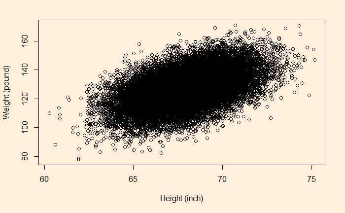
Let’s use the human height vs weight dataset to understand the concept of regression. The dataset has 25,000 synthetic records of human heights and weights of 18-year-old children. These were simulated from a 1993 Growth Survey of 25,000 children from birth to 18 years of age recruited from Maternal and Child Health Centres and schools.

Now, build a linear regression between the height and the weight by running the following R code.
lm(hw_data$Weight.Pounds. ~ hw_data$Height.Inches.)It gives the following output.
Call:
lm(formula = hw_data$Weight.Pounds. ~ hw_data$Height.Inches.)

Coefficients:
           (Intercept)  hw_data$Height.Inches.
               -82.576                   3.083
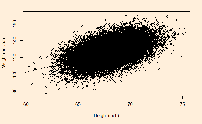
So the equation becomes weight = 3.083 x height – 82.576. You can add the line (the regression line) to the plot by typing,
abline(lm(hw_data$Weight.Pounds. ~ hw_data$Height.Inches.))
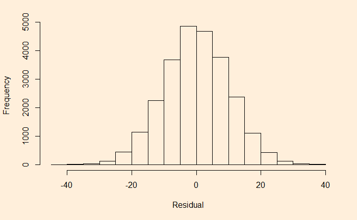
The residuals must follow a Gaussian if the data is random and independent. Let’s get the residual and make a histogram.
hist(hw_data$Weight.Pounds. - ( -82.576 + 3.083 * hw_data$Height.Inches.), main = "", xlab = "Residual", ylab = "Frequency")

