If Lebron has a 75% success rate from free throws, what is the chance that he makes nine or above out of 10 from the free throw line in the next game? We know how to solve this problem. Just apply the binomial relationship and estimate. Estimate the probability of nine and ten successes, and add them up. Like this:
10C9 x (0.75)9 x (0.25)1 + 10C10 x (0.75)10 x (0.25)0 = 0.244
Three Games of Basketball
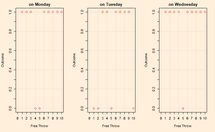
Obviously, you can not have 24.4% of doing something in a match – you either do it 100% or not do it at all. Let’s get into details of what these mean – using a few R functions and visualisations. Let’s look at three instances of Lebron throwing a total of ten, at the success rate of 0.75. Run the following R code:
trial <- 10
xxx <- seq(1,trial)
prob_x <- 0.75

game_play <- function(n){
  sample(c(0,1),size = 1, replace = TRUE,prob = c((1-prob_x), prob_x))
  }

xtick<-seq(0, trial, by= 1)
ytick<-seq(0, 1, by=0.1)


par(bg = "antiquewhite1", mfrow = c(1,3))
plot(xxx, sapply(xxx, game_play), xlim = c(0,trial), ylim = c(0,1), xlab="Free Throw", ylab="Outcome", col = "red", cex = 1, pch = 5, type = "p", bg=23, main="on Monday")
grid()
axis(side=1, at=xtick, labels = TRUE)
axis(side=2, at=ytick, labels = FALSE)

plot(xxx, sapply(xxx, game_play), xlim = c(0,trial), ylim = c(0,1), xlab="Free Throw", ylab="Outcome", col = "red", cex = 1, pch = 5, type = "p", bg=23, main="on Tuesday")
grid()
axis(side=1, at=xtick, labels = TRUE)
axis(side=2, at=ytick, labels = FALSE)

plot(xxx, sapply(xxx, game_play), xlim = c(0,trial), ylim = c(0,1), xlab="Free Throw", ylab="Outcome", col = "red", cex = 1, pch = 5, type = "p", bg=23, main="on Wednesday")
grid()
axis(side=1, at=xtick, labels = TRUE)
axis(side=2, at=ytick, labels = FALSE)
He made it on Wednesday; on Tuesday and Monday, he didn’t. We used an R function called sample, a random sample generator coupled with a probability condition of 0.75 for success. Each time you run this code, you get three plots with different outcomes.
PMF and CDF
You must have heard about Probability Mass Functions, Cumulative Density Functions etc. They are pretty handy to understand more about the winning chances in distributions, and we will use them to answer the original question.
Let’s place three plots side by side. The one on the left is what could happen in an actual game. The one on its right is a plot of chances for each try if you play the game several times, and the one on the extreme right is the plot of the cumulative probability distribution. You can get cumulative by adding the probabilities in the PMF one by one, from left to right.

Now let us answer the original question by looking at the plot. The one on the left is the least useful to make any conclusions. If you look at this one-off game, you may presume that Lebron would not make 9 or 10 in a game. It is the answer by someone who saw only one game or has scant regard for statistics!
Calculating from the PMF plot is simple: add the density at nine successful shots and ten successful shots together (I have marked 9 with a vertical line as a guide). And 0.188 + 0.056 = 0.244. Using the last plot (CDF), you calculate everything above 8. Or subtract from 1, the number corresponding to 8; you get 1 – 0.756 = 0.244.

