The outcome variable in survival analysis is the time until an event occurs. Since studies are often time-bounded, some patients may survive the event at the end of the study, and others may stop responding to the survey midway through. In either case, those patients’ survival times are censored. As censored patients also provide valuable data, the analyst gets into a dilemma of whether to discard those candidates.
Let’s examine five patients in a study. The filled circles represent the completion of the event (e.g., death), and the open circles represent the censoring (either dropping out or surviving the study’s end date).

The survival function, S(t), is the probability that the true survival time (T) exceeds some fixed number t.
S(t) = P(T > t)
S(t) decreases with time (t) as the probability decreases as time passes.
In the above example, how do you conclude the probability of surviving 300 days, S(300)? Will it be 1/3 = 0.33 (only the one survived out of three events, ignoring the censored) or 3/5 = 0.6 (assuming the censored candidates also survived)? What difference does it make to the conclusion that one of them dropped out early when she was too sick?
Kaplan and Meier came up with a smart solution to this. Note that they worked on this problem separately. Their survival curve is made the following way.
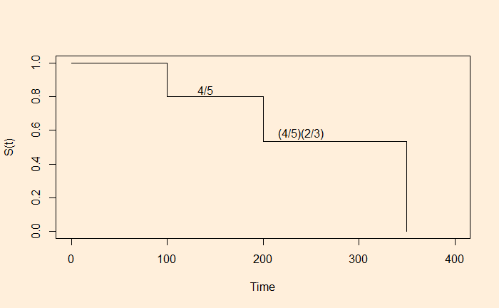
1) The first event happened at time 100. The probability of survival at t = 100 is 4/5, noting that four of the five patients were known to have survived that stage.

2) We now proceed to the next event, patient 3. Note that we skipped the censored time of patient 2.

Now, two out of three survived. The overall survival probability at t = 200 is (4/5) x (2/3).
3) Move to the last event (patient 5); the survival function is zero ((4/5) x (2/3) x 0). This leads to the Kaplan -Meier plot:


