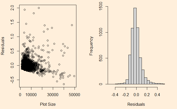
We have seen it before; the residuals in linear regression must be random and independent. It also means that the residuals are scattered around a mean with constant variance. This is known as homoscedasticity. When that is violated, it’s heteroscedasticity.
Here is the (simulated) height weight data from the UCLA statistics, with the regression line.
model <- lm(Wt.Pounds ~ Ht.Inch, data=H_data)
plot(H_data$Ht.Inch , H_data$Wt.Pounds, xlab = "Height (Inches)", ylab = "Weight (Pounds)")
abline(model, col = "deepskyblue3")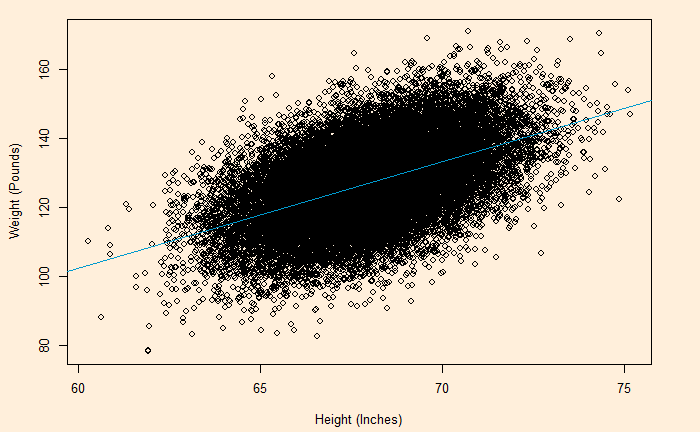
We will do a residual plot, a collection of points corresponding to the distances from the best-fit line.
H_data$resid <- resid(model)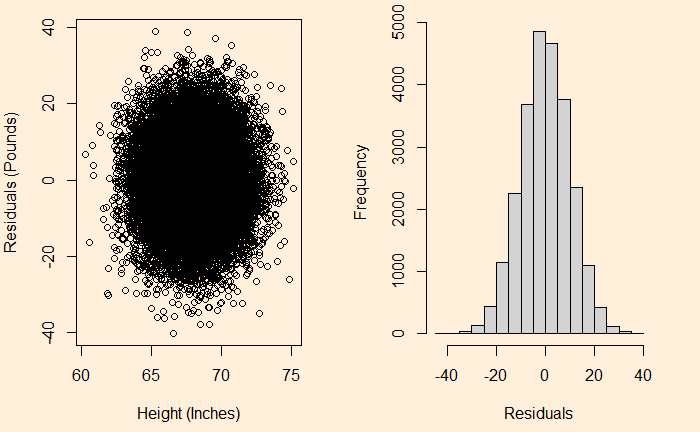
On the other hand, see the plot of sale price vs property area.
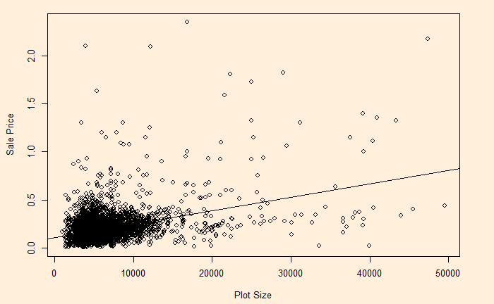
The relationship has heteroscedasticity, as evident from the skewness of residual towards one side.
