We have seen how the R package ‘tigerstats’ can help visualise basic statistics. The library has several functions and datasets to teach statistics at an elementary level. We will see a couple of them that enable hypothesis testing.
chi-square test
We start with a test for Independence using the chi-square test. The example is the same as we used previously. Here, we create the database with the following summary.
| High School | Bachelors | Masters | Ph.d. | Total | |
| Female | 60 | 54 | 46 | 41 | 201 |
| Male | 40 | 44 | 53 | 57 | 194 |
| Total | 100 | 98 | 99 | 98 | 395 |
as_tibble(educ)
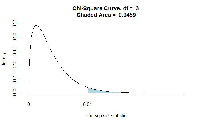
The function to use is ‘chisqtestGC’, which takes two variables (~var1 + var2) to test their association. Additional attributes such as graph and verbose yield the relevant graph (ch-square curve) for the P-value and details of the output.
chisqtestGC(~EDU+SEX, data=educ, graph = TRUE, verbose = TRUE)Pearson's Chi-squared test
Observed Counts:
SEX
EDU Female Male
Bachelors 54 44
High School 60 40
Masters 46 53
Ph.d. 41 57
Counts Expected by Null:
SEX
EDU Female Male
Bachelors 49.87 48.13
High School 50.89 49.11
Masters 50.38 48.62
Ph.d. 49.87 48.13
Contributions to the chi-square statistic:
SEX
EDU Female Male
Bachelors 0.34 0.35
High School 1.63 1.69
Masters 0.38 0.39
Ph.d. 1.58 1.63
Chi-Square Statistic = 8.0061
Degrees of Freedom of the table = 3
P-Value = 0.0459 
Binomial test for proportion
Suppose a coin toss landed on 40 heads in 100 attempts. Perform a two-sided hypothesis test for p = 0.5 as the Null.
binomtestGC(x=40,n=100,p=0.5, alternative = "two.sided", graph = TRUE, conf.level = 0.95)x = variable under study
n = size of the sample
p = Null Hypothesis value for population proportion
alternative = takes “two.sided”, “less” or “greater” for the computation of the p-value.
conf.level = number between 0 and 1, indicating the confidence interval
graph = If TRUE, plot graph of p-value
Exact Binomial Procedures for a Single Proportion p:
	Results based on Summary Data

Descriptive Results:  40 successes in 100 trials

Inferential Results:

Estimate of p:	 0.4
SE(p.hat):	 0.049

95% Confidence Interval for p:

          lower.bound         upper.bound
          0.303295            0.502791

Test of Significance:

	H_0:  p = 0.5
	H_a:  p != 0.5

P-value: P = 0.0569 
binomtestGC(x=40,n=100,p=0.5, alternative = "less", graph = TRUE, conf.level = 0.95)
Exact Binomial Procedures for a Single Proportion p:
	Results based on Summary Data

Descriptive Results:  40 successes in 100 trials

Inferential Results:

Estimate of p:	 0.4
SE(p.hat):	 0.049

95% Confidence Interval for p:

          lower.bound         upper.bound
          0.000000            0.487024

Test of Significance:

	H_0:  p = 0.5
	H_a:  p < 0.5

P-value: P = 0.0284 
