Employee Attrition Dataset

We continue using the ‘tigerstats’ package to analyse the ‘IBM HR Analytics Employee Attrition & Performance’ dataset, a fictional data set created by IBM data scientists and taken from Kaggle. The dataset contains various parameters related to attribution,

Em_data <- read.csv("D:/04Compute/Web/Employee-Attrition.csv")
str(Em_data)

'data.frame':	1470 obs. of  35 variables:
 $ Age                     : int  41 49 37 33 27 32 59 30 38 36 ...
 $ Attrition               : chr  "Yes" "No" "Yes" "No" ...
 $ BusinessTravel          : chr  "Travel_Rarely" "Travel_Frequently" "Travel_Rarely" "Travel_Frequently" ...
 $ DailyRate               : int  1102 279 1373 1392 591 1005 1324 1358 216 1299 ...
 $ Department              : chr  "Sales" "Research & Development" "Research & Development" "Research & Development" ...
 $ DistanceFromHome        : int  1 8 2 3 2 2 3 24 23 27 ...
 $ Education               : int  2 1 2 4 1 2 3 1 3 3 ...
 $ EducationField          : chr  "Life Sciences" "Life Sciences" "Other" "Life Sciences" ...
 $ EmployeeCount           : int  1 1 1 1 1 1 1 1 1 1 ...
 $ EmployeeNumber          : int  1 2 4 5 7 8 10 11 12 13 ...
 $ EnvironmentSatisfaction : int  2 3 4 4 1 4 3 4 4 3 ...
 $ Gender                  : chr  "Female" "Male" "Male" "Female" ...
 $ HourlyRate              : int  94 61 92 56 40 79 81 67 44 94 ...
 $ JobInvolvement          : int  3 2 2 3 3 3 4 3 2 3 ...
 $ JobLevel                : int  2 2 1 1 1 1 1 1 3 2 ...
 $ JobRole                 : chr  "Sales Executive" "Research Scientist" "Laboratory Technician" "Research Scientist" ...
 $ JobSatisfaction         : int  4 2 3 3 2 4 1 3 3 3 ...
 $ MaritalStatus           : chr  "Single" "Married" "Single" "Married" ...
 $ MonthlyIncome           : int  5993 5130 2090 2909 3468 3068 2670 2693 9526 5237 ...
 $ MonthlyRate             : int  19479 24907 2396 23159 16632 11864 9964 13335 8787 16577 ...
 $ NumCompaniesWorked      : int  8 1 6 1 9 0 4 1 0 6 ...
 $ Over18                  : chr  "Y" "Y" "Y" "Y" ...
 $ OverTime                : chr  "Yes" "No" "Yes" "Yes" ...
 $ PercentSalaryHike       : int  11 23 15 11 12 13 20 22 21 13 ...
 $ PerformanceRating       : int  3 4 3 3 3 3 4 4 4 3 ...
 $ RelationshipSatisfaction: int  1 4 2 3 4 3 1 2 2 2 ...
 $ StandardHours           : int  80 80 80 80 80 80 80 80 80 80 ...
 $ StockOptionLevel        : int  0 1 0 0 1 0 3 1 0 2 ...
 $ TotalWorkingYears       : int  8 10 7 8 6 8 12 1 10 17 ...
 $ TrainingTimesLastYear   : int  0 3 3 3 3 2 3 2 2 3 ...
 $ WorkLifeBalance         : int  1 3 3 3 3 2 2 3 3 2 ...
 $ YearsAtCompany          : int  6 10 0 8 2 7 1 1 9 7 ...
 $ YearsInCurrentRole      : int  4 7 0 7 2 7 0 0 7 7 ...
 $ YearsSinceLastPromotion : int  0 1 0 3 2 3 0 0 1 7 ...
 $ YearsWithCurrManager    : int  5 7 0 0 2 6 0 0 8 7 ...

barchartGC

barchartGC(~Gender,data=Em_data)

barchartGC(~Attrition+Gender,data=Em_data, stack = TRUE)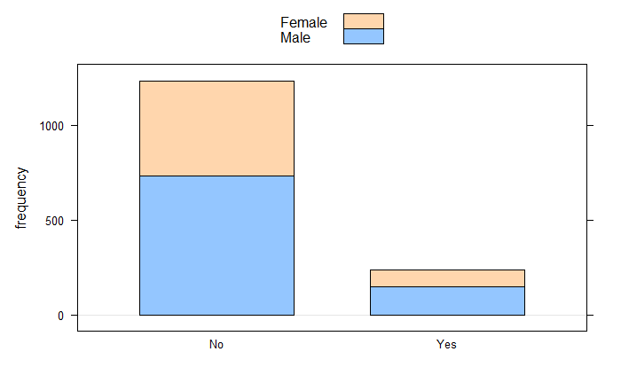

xtabs

xtabs(~Attrition+MaritalStatus,data=Em_data)

         MaritalStatus
Attrition Divorced Married Single
      No       294     589    350
      Yes       33      84    120

xtabs(~Attrition+Gender,data=Em_data)

         Gender
Attrition Female Male
      No     501  732
      Yes     87  150

CIMean

CIMean(~MonthlyIncome,data=Em_data)

ttestGC

ttestGC(~MonthlyIncome,data=Em_data)

Inferential Procedures for One Mean mu:

Descriptive Results:

variable       mean     sd       n          
MonthlyIncome  6502.931 4707.957 1470       

Inferential Results:

Estimate of mu:	 6503 
SE(x.bar):	 122.8 

95% Confidence Interval for mu:

          lower.bound         upper.bound          
          6262.062872         6743.799713      

ttestGC(~Age,data=Em_data)

Inferential Procedures for One Mean mu:

Descriptive Results:

variable  mean     sd       n          
Age       36.924   9.135    1470       

Inferential Results:

Estimate of mu:	 36.92 
SE(x.bar):	 0.2383 

95% Confidence Interval for mu:

          lower.bound         upper.bound          
          36.456426           37.391193