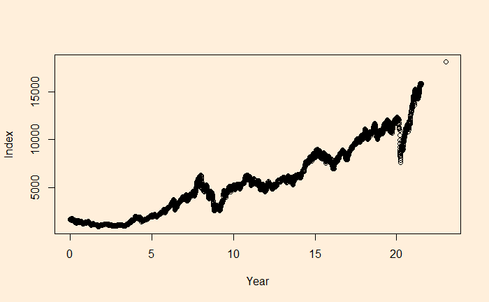
We have seen examples of regression where the basic assumption of uncorrelated residuals is compromised. Finding the autocorrelation of the residuals using Durbin–Watson is one way to diagnose the correlation. Here, we perform a step-by-step estimation.
Step 1: Plot the data
plot(Nif_data$Year, Nif_data$Index, xlab = "Year", ylab = "Index")
Step 2: Develop a regression model
fit <- lm(Index ~ Year, data=Nif_data)
summary(fit)
Call:
lm(formula = Index ~ Year, data = Nif_data)
Residuals:
Min 1Q Median 3Q Max
-3410.3 -544.5 -96.5 507.6 5603.0
Coefficients:
Estimate Std. Error t value Pr(>|t|)
(Intercept) -438.128 27.801 -15.76 <2e-16 ***
Year 566.726 2.243 252.65 <2e-16 ***
---
Signif. codes: 0 ‘***’ 0.001 ‘**’ 0.01 ‘*’ 0.05 ‘.’ 0.1 ‘ ’ 1
Residual standard error: 1020 on 5352 degrees of freedom
Multiple R-squared: 0.9226, Adjusted R-squared: 0.9226
F-statistic: 6.383e+04 on 1 and 5352 DF, p-value: < 2.2e-16Step 3: Estimate Residuals
Nif_data$resid <- resid(fit)Step 4: Durbin–Watson (D-W) Statistics
D-W statistic is the sum of differences between successive residuals squared divided by the sum of residuals squared.
D-W Statistics = sum (ei - ei-1)2 / sum(ei2)sum(diff(Nif_data$resid)^2) / sum(Nif_data$resid^2)0.006301032R can do better – using the ‘durbinWatsonTest’ function from the library ‘car’.
library(car)
fit <- lm(Index ~ Year, data=Nif_data)
durbinWatsonTest(fit)
lag Autocorrelation D-W Statistic p-value
1 0.9936623 0.006301032 0
Alternative hypothesis: rho != 0
