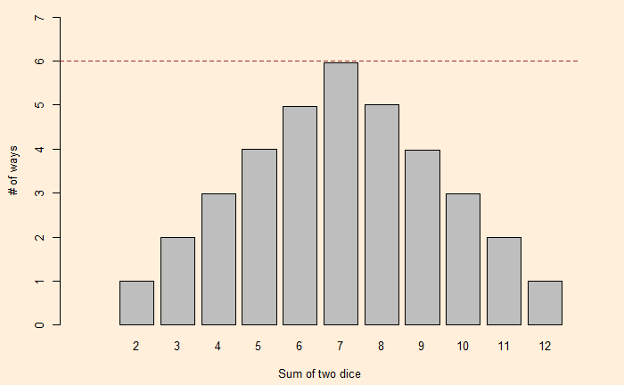
We have seen how one can describe a die with a polynomial. As a well-known example, i.e., the roll of two (regular) dice. The expected probabilities on the sum of dice are:
f(x) x f(x)= (x6 + x5 + x4 + x3 + x2 + x1) (x6 + x5 + x4 + x3 + x2 + x1)
x12 + 2x11 + 3x10 + 4x9 + 5x8 + 6x7 + 5x6 + 4x5 + 3x4 + 2x3 + x2

Where the exponents of x are the X-values and coefficients of x are the Y-values.
Now, a question arises: Can we find another pair of two dice with the same distribution for the sums? One way to find out is to factorise the polynomial, x12 + 2x11 + 3x10 + 4x9 + 5x8 + 6x7 + 5x6 + 4x5 + 3x4 + 2x3 + x2. George Sicherman discovered that another pair of numbers can lead to the same outcome. They are:
f(x) x g(x)= (x4 + x3 + x3 + x2 + x2 + x1) (x8 + x6 + x5 + x4 + x3 + x1)
They represent two cubes with the following numbering.
Cube 1: 1, 2, 2, 3, 3, 4
Cube 2: 1, 3, 4, 5, 6, 8
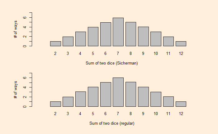
Let’s roll these dice a million times and find out.
dice_1 <- c(1, 2, 2, 3, 3, 4)
dice_2 <- c(1, 3, 4, 5, 6, 8)
prob_1 <- rep(1/6,6)
prob_2 <- rep(1/6,6)

itr <- 1000000

toss <- replicate(itr, {
sam1 <- sample(dice_1, 1, prob = prob_1, replace = TRUE)
sam2 <- sample(dice_2, 1, prob = prob_2, replace = TRUE)
sam <- sam1 + sam2
})
Here is the comparison of a pair of Sicherman dice with the regular.


