We have seen estimating the variance inflation factor (VIF) is a way of detecting multicollinearity during regression. This time, we will work out one example using the data frame from “Statistics by Jim”. We will use R programs to execute the regressions.
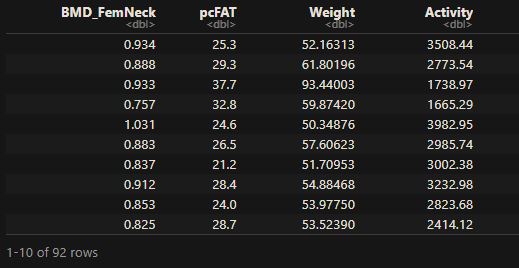
This regression will model the relationship between the dependent variable (Y), the bone mineral density of the femoral neck, and three independent variables (Xs): physical activity, body fat percentage, and weight. The first few lines of the data are below:

The objective of the regression is to find the best (linear) model that fits BMD_FemNeck with pcFAT, Weight, and Activity.
model <- lm(BMD_FemNeck ~ pcFAT + Weight + Activity, data=M_data)
summary(model)
Call:
lm(formula = BMD_FemNeck ~ pcFAT + Weight + Activity, data = M_data)
Residuals:
Min 1Q Median 3Q Max
-0.210260 -0.041555 -0.002586 0.035086 0.213329
Coefficients:
Estimate Std. Error t value Pr(>|t|)
(Intercept) 5.214e-01 3.830e-02 13.614 < 2e-16 ***
pcFAT -4.923e-03 1.971e-03 -2.498 0.014361 *
Weight 6.608e-03 9.174e-04 7.203 1.91e-10 ***
Activity 2.574e-05 7.479e-06 3.442 0.000887 ***
---
Signif. codes: 0 ‘***’ 0.001 ‘**’ 0.01 ‘*’ 0.05 ‘.’ 0.1 ‘ ’ 1
Residual standard error: 0.07342 on 88 degrees of freedom
Multiple R-squared: 0.5201, Adjusted R-squared: 0.5037
F-statistic: 31.79 on 3 and 88 DF, p-value: 5.138e-14The relationship will be:
5.214e-01 – 4.923e-03 x pcFAT + 6.608e-03 x Weight + 2.574e-05 x Activity
To estimate each VIF value, we will first consider the corresponding X value as the dependent variable (against the remaining Xs as the independent variables), do regression and evaluate the R-squared.
body fat percentage (pcFAT)
summary(lm(pcFAT ~ Weight + Activity , data=M_data))Call:
lm(formula = pcFAT ~ Weight + Activity, data = M_data)
Residuals:
Min 1Q Median 3Q Max
-7.278 -2.643 -0.650 2.577 11.421
Coefficients:
Estimate Std. Error t value Pr(>|t|)
(Intercept) 6.5936609 1.9374973 3.403 0.001 **
Weight 0.3859982 0.0275680 14.002 <2e-16 ***
Activity 0.0004510 0.0003993 1.129 0.262
---
Signif. codes: 0 ‘***’ 0.001 ‘**’ 0.01 ‘*’ 0.05 ‘.’ 0.1 ‘ ’ 1
Residual standard error: 3.948 on 89 degrees of freedom
Multiple R-squared: 0.6879, Adjusted R-squared: 0.6809
F-statistic: 98.1 on 2 and 89 DF, p-value: < 2.2e-16The R-squared is 0.6879, and the VIF for pcFAT is:
1/(1-0.6879) = 3.204101
weight (Weight )
summary(lm(Weight ~ pcFAT + Activity , data=M_data))Call:
lm(formula = Weight ~ pcFAT + Activity, data = M_data)
Residuals:
Min 1Q Median 3Q Max
-26.9514 -5.1452 -0.5356 5.1606 24.0891
Coefficients:
Estimate Std. Error t value Pr(>|t|)
(Intercept) 6.3369837 4.3740142 1.449 0.151
pcFAT 1.7817966 0.1272561 14.002 <2e-16 ***
Activity -0.0012905 0.0008532 -1.513 0.134
---
Signif. codes: 0 ‘***’ 0.001 ‘**’ 0.01 ‘*’ 0.05 ‘.’ 0.1 ‘ ’ 1
Residual standard error: 8.482 on 89 degrees of freedom
Multiple R-squared: 0.6914, Adjusted R-squared: 0.6845
F-statistic: 99.69 on 2 and 89 DF, p-value: < 2.2e-16The R-squared is 0.6914, and the VIF for Weight is 1/(1-0.6914) = 3.240441
physical activity (Activity)
summary(lm(Activity ~ Weight + pcFAT, data=M_data))Call:
lm(formula = Activity ~ Weight + pcFAT, data = M_data)
Residuals:
Min 1Q Median 3Q Max
-1532.8 -758.9 -168.0 442.6 4648.7
Coefficients:
Estimate Std. Error t value Pr(>|t|)
(Intercept) 2714.42 460.34 5.897 6.56e-08 ***
Weight -19.42 12.84 -1.513 0.134
pcFAT 31.33 27.74 1.129 0.262
---
Signif. codes: 0 ‘***’ 0.001 ‘**’ 0.01 ‘*’ 0.05 ‘.’ 0.1 ‘ ’ 1
Residual standard error: 1041 on 89 degrees of freedom
Multiple R-squared: 0.02556, Adjusted R-squared: 0.003658
F-statistic: 1.167 on 2 and 89 DF, p-value: 0.316
1/(1-0.02556) = 1.02623
VIF Function in R
The calculations can be simplified using the function VIF in ‘regclass’ package.
model <- lm(BMD_FemNeck ~ pcFAT + Weight + Activity, data=M_data)
VIF(model)
pcFAT Weight Activity
3.204397 3.240334 1.026226 All three VIF values remain reasonably low (< 10); therefore, we don’t suspect collinearity in these three variables.

