Suppose a drug was tested on eight people. Five people became better, and three did not. How do we know if the drug works? Naturally, eight is far from the population of a region, which could be in the thousands.
The bootstrapping technique fundamentally pretends that the sample histogram is the population histogram. It then performs repeated sampling (with replacement) from the collected dataset. It creates histograms of outcome statistics of what might have been obtained if the experiment had been done several times.
Here are the eight data collected. The positive values correspond to people who improved with the drug, and the negative values are the opposite.
data <- c(-3.5, -3.0, -1.8, 1.4, 1.6, 1.7, 2.9, 3.5)Let’s randomly sample from this a hundred times, estimate the mean each time and plot the histogram of it.
resamples <- lapply(1:100, function(i) sample(data, replace = T))
boot.mean <- sapply(resamples, mean)
hist(boot.mean, breaks = 20)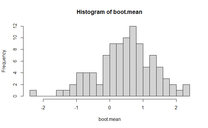
Note that when randomly sampling from the dataset, some data can come multiple times; therefore, we see the histogram (distribution) of the mean.

