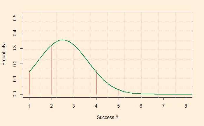
We have seen it before: what is the chance of getting three heads if you toss a coin five times? The answer is about 30%. You know how to do it: 5C3 (0.5)3(0.5)5-3 = 0.3125. The distribution representing the probability of each success when a coin is tossed five times is given by the PMF of binomial.

We have used the following R code (the dbinom function for PMF) to generate this plot.
xx <- seq(1,30,1)
p <- 0.5
q = 1 - p
toss <- 5

par(bg = "antiquewhite1")
plot(dbinom(xx,race,p), xlim = c(1,8), ylim = c(0,0.52), xlab="Success #", ylab="Probability", cex = 1, pch = 5, type = "h", main="", col = ifelse(xx >= 24,"#006600",'red'))
If you look at the distribution carefully, you will see that it resembles a normal distribution. For the normal distribution, we need a mean and a standard deviation. The mean is easy: you multiply the total number of tossing with the probability of success in one toss, i.e., 5 x 0.5 = 2.5. The variance of a binomial distribution is N x p x (1-p); the standard deviation is its square root. Let’s try making a normal distribution and superpose.
xx <- seq(1,30,1)
p <- 0.5
q = 1 - p
toss <- 5

par(bg = "antiquewhite1")
plot(dbinom(xx,toss,p), xlim = c(1,8), ylim = c(0,0.52), xlab="Success #", ylab="Probability", cex = 1, pch = 5, type = "h", main="", col = ifelse(xx >= 24,"#006600",'red'))

xx <- seq(1,30,0.1)
mean_i <- toss*p
sd_i <- sqrt(toss*p*q)

lines(xx, dnorm(xx, mean = mean_i , sd = sd_i ), xlim = c(0,30), ylim = c(0,0.2), xlab="Evidence for guilt", ylab="Frequency", col = "springgreen4", cex = 1, pch = 5, type = "l", bg=23, lwd = 2, main="")
grid(nx = 10, ny = 9)

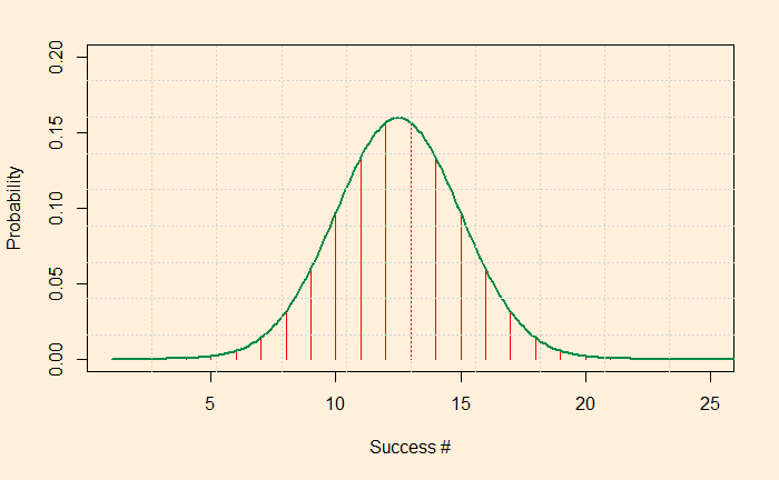
Looks like the green line representing the normal distribution is almost passing through binomial values. We will soon see that when the number of trials (N) is large, the binomial becomes indistinguishable from a normal distribution. For N is 25. Like this:


