We have seen Berkson’s paradox before. It’s an erroneous correlation attributed to surveys done under specific conditions. Here we simulate a situation using R codes and illustrate the paradox.
Let’s assume a college admission process that involves two tests – test 1 and test 2. We create a set of random numbers with a positive correlation between Mark 1 and Mark 2.
x <- 1:100
y <- x + rnorm(100, 100,50)

plot(x,y, xlim = c(0,100), ylim = c(0,300),  frame.plot=FALSE, xlab = "Mark 1", ylab = "Mark 2")
text(paste("Correlation:", round(cor(x, y), 2)), x = 40, y = 10)
You will see that a reasonable positive correlation exists between the marks of the two tests (correlation coefficient = + 0.42).
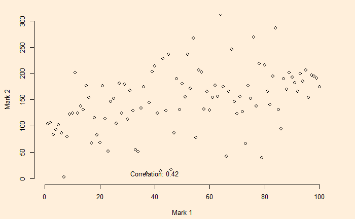
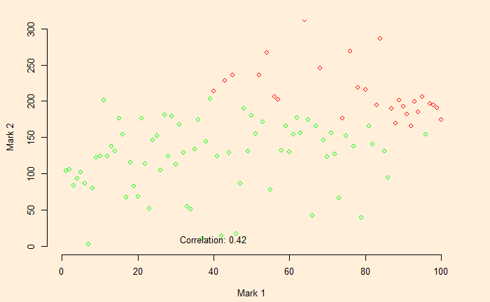
Now, we impose a cut-off for the selection, i.e., the total marks (test 1 and test 2) of more than 250 to be eligible for admission.
plot(x,y, xlim = c(0,100), ylim = c(0,300),  frame.plot=FALSE,  col = ifelse(x + y > 250 ,'red','green'), xlab = "Mark 1", ylab = "Mark 2")
text(paste("Correlation:", round(cor(x, y), 2)), x = 40, y = 10)
And the eligible candidates are denoted by red circles.
Pick the red dots – the candidates who fulfilled the minimum criterion of total marks > 250 – separate and plot.
total <- data.frame(x = x, y = y, z = x+y)
total <- total %>% filter(z > 250)

plot(total$x, total$y, xlab = "Mark 1", ylab = "Mark 2", xlim = c(0,100), ylim = c(0,300))
text(paste("Correlation:", round(cor(total$x, total$y), 2)), x = 40, y = 130)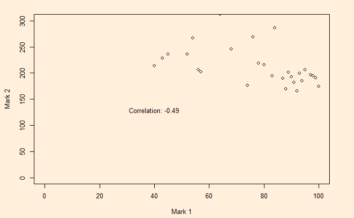
If one surveys this college, there is a chance that the results find a negative correlation between performance in test 1 vs test 2 (in this case, a correlation of – 0.49). Imagine the first subject was science and the second was humanities! People might even attach causalities to the observations, which are biased by the selection criteria.
