Poisson, Gamma and the Objective
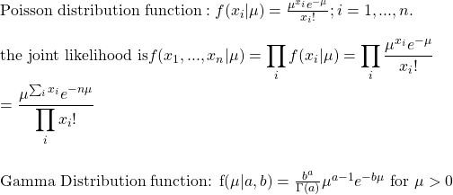
Last time we set the objective: i.e. to find the posterior distribution of the expected value, from a Poisson distributed set of variables using a Gamma distribution of the mean as the prior information.
Caution: Math Ahead!

So we have a function and a prior. We will obtain the posterior using Bayes’ theorem.

The integral in the denominator will be a constant. Therefore,
![]()
Look at the above equation carefully. Don’t you see the resemblance with a Gamma p.d.f, sans the constant?
![]()
End Game
So if you know a prior gamma, you can get a posterior gamma based on the above equations. Recall the table from the previous post. The Sum of xi is 42000 and n is 7. Assume Gamma(6000,1) as a prior. This leads to a posterior of Gamma( 48000,8). Mean = 48000/8 and variance = 48000/82. The standard error becomes the square root of variance divided by the square root of n.

Expanding the Prior Landscape
Naturally, you may be wondering why I chose a prior that has a mean of 6000, or where I got that distribution from etc. And these are valid arguments. The prior was arbitrarily chosen to perform the calculations. In reality, you can get it from several sources – from similar shops in the town, scenarios created for worst (or best) case situations and so on. Rule number one in the scientific process is to challenge, and two is to experiment. So, we run a few cases and see what happens.
Imagine you come up with a prior of Gamma(8000,2). What does this mean? A distribution with a mean of 4000 and a variance of 2000 (standard deviation 44). [Recall mean = a/b; variance = a/b2 ]. The original distribution (Poisson) remains the same because it is your data.

Take another, Gamma(8000,1). A distribution with a mean of 8000 and a variance of 8000 (standard deviation 89).

Yes, the updated distributions do change positions, but they still hang around the original (from own data) probability density created by the Poisson function.
You may have noticed the power of Bayesian inference. The prior information can change expectations on the future yet retain the core elements.

