As we have seen, autocorrelation is the correlation of a variable in a time series with itself but at a time lag. For example, how are the variables at time ts correlated to the t-1s? We will use the aus_production dataset from the R library ‘fpp3’ to illustrate the concept of autocorrelation.
library(fpp3)
str(aus_production)
$ Quarter : qtr [1:74] 1992 Q1, 1992 Q2, 1992 Q3, 1992 Q4, 1993 Q1, 1993 Q2, 1993 Q3, 1993 Q4, 1994 Q1, 1994 Q2, 1994 Q3, 1994 Q4, 1995 Q1, 1995 Q2, 1995 Q3,...
$ Beer : num [1:74] 443 410 420 532 433 421 410 512 449 381 ...
$ Tobacco : num [1:74] 5777 5853 6416 5825 5724 ...
$ Bricks : num [1:74] 383 404 446 420 394 462 475 443 421 475 ...
$ Cement : num [1:74] 1289 1501 1539 1568 1450 ...
$ Electricity: num [1:74] 38332 39774 42246 38498 39460 ...
$ Gas : num [1:74] 117 151 175 129 116 149 163 138 127 159 ...
We will use the beer production data.
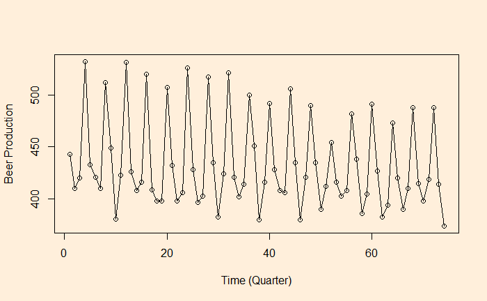
Let’s plot the production data with itself without any lag in time.
plot(B_data, B_data, xlab = "Beer Production at i", ylab = "Beer Production at i")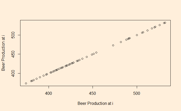
There is no surprise here; the data is in perfect correlation. In the next step, we will give a lag of one time interval, i.e., a plot of (2,1), (3,2), (4,3), etc. The easiest way to achieve this is to remove the first element of the vector and plot against the vector with the last element removed.

plot(B_data[-1], B_data[-n], xlab = "Beer Production at i - 1", ylab = "Beer Production at i")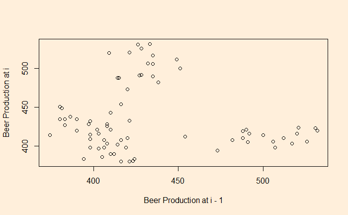
You clearly see a lack of correlation. What about a plot with a lag of 2 and 4?
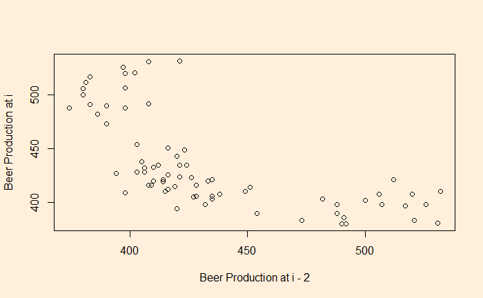
There is a negative correlation compared with the time series 2 quarters ago.
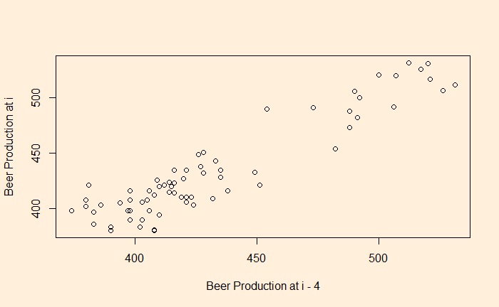
There is a good correlation compared with the time series 4 quarters ago.
The whole process is established using the autocorrelation function (ACF).
autocorrelation <- acf(B_data, lag.max=10, plot=FALSE)
plot(autocorrelation,
     main="Autocorrelation",
     xlab="Lag Parameter",
     ylab="ACF")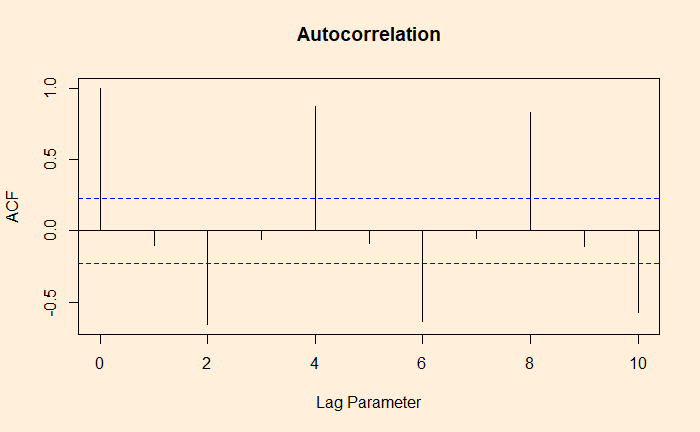
ACF at large parameter 1 indicates how successive values of beer production relate to each other, 2 indicates how production two periods apart relate to each other, etc.
