Areas through Monte Carlo

You may have known how to evaluate a definite integral or integrals bounded within limits. For example, consider the following:

$\int_0^1 x^2 dx$

We can estimate the value by integrating the function y = x² and applying the limits.

$\int_0^1 x^2 dx = \frac{x^3}{3}|_0^1 = \frac{1}{3}$

The function (within those bounds) is plotted below, and the required integral is the area under the curve.

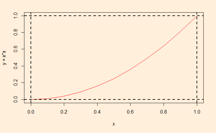
Looking at the graph above, one can envision that the required area is the fraction of a unit square at which the relationship, y </= x² works. As we have done before, we will fill the unit square by selecting random numbers between 0 and 1 and collect the fraction that obeys the equation. This this:

itr <- 10000

xxx <- replicate(itr,0)
yyy <- replicate(itr,0)
counter <- 0

for (rep_trial in 1:itr) {
  
  xx <- runif(1)
  yy <- runif(1)
  if(yy <= xx*xx){
    xxx[rep_trial] <- xx
    yyy[rep_trial] <- yy
    counter <- counter + 1
  }
}
counter/itr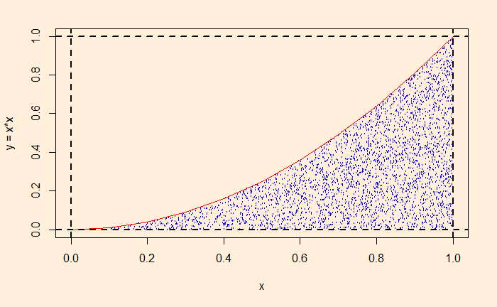

And the output (the integral, counter/itr) is 0.3312.

Simulations like these, the probability of hitting between the restricted boundaries of a unit square, are handy for estimating areas under functions that are difficult to integrate analytically.

Related Posts