The last time we did random sampling and counting, also known as the Monte Carlo experiments. Today we build two programs to demonstrate what is called the law of large numbers through two examples, coin tossing and die rolling. In case you forgot, the law of large numbers is a phenomenon where the actual value starts converging to the expected value as the number of events increases.
Coin Toss
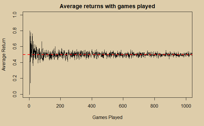
Imagine you are in a coin game: you get 1 dollar for a head and nothing for a tail. What is the average amount you are gaining from the play? We create an R program that calculates the average of several sampling outcomes and plots it as a function of the number of games played.
fin_number <- 1000
xx <- replicate(fin_number,0) # initiating vector
yy <- replicate(fin_number,0) # initiating vector

for (rep_trial in 1:fin_number) {

win_fr <- replicate(rep_trial, {
  try <- sample(c(1,0), size = 1, replace = TRUE, prob = c(0.5,0.5))
  })
 xx[rep_trial] <- rep_trial
 yy[rep_trial] <- mean(win_fr)
}


par(bg = "#decdaa")
plot(xx,yy, type = "l", main = "Average returns with games played", xlab = "Games Played", ylab = "Average Return", xlim = c(0,1000), ylim = c(0,1))
abline(h = 0.5, col="red", lwd=2, lty=2)
The code uses four functions in R – for loop, replicate, sample and plot. The red dotted line represents the expected probability of 0.5 for a head in coin-tossing.
Dice Roll
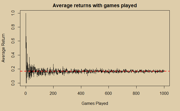
In this game, you get one point when you roll a 1, nothing otherwise.
fin_number <- 1000
xx <- replicate(fin_number,0)
yy <- replicate(fin_number,0)

for (rep_trial in 1:fin_number) {

win_fr <- replicate(rep_trial, {
  die_cast <- sample(c(1,2,3,4,5,6), size = 1, replace = TRUE, prob = c(1/6, 1/6, 1/6, 1/6, 1/6, 1/6))
if (die_cast == 1) {
  counter = 1
} else {
  counter = 0
}
  })

xx[rep_trial] <- rep_trial
yy[rep_trial] <- mean(win_fr)

}

par(bg = "#decdaa")
plot(xx,yy, type = "l", main = "Average returns with games played", xlab = "Games Played", ylab = "Average Return", xlim = c(0,1000), ylim = c(0,1))
abline(h = 1/6, col="red", lwd=2, lty=2)
You know the probability of obtaining a 1 from the rolling of a fair die is (1/6), which is represented in the figure by the red dotted line.
The Roulette
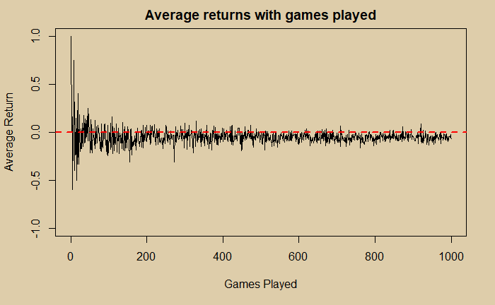
I can not stop this post without referring to Roulette. Here is what we obtain, by setting probabilities to (18/38) and (20/38) for winning 1 and -1, respectively.
fin_number <- 1000
xx <- replicate(fin_number,0)
yy <- replicate(fin_number,0)

for (rep_trial in 1:fin_number) {

win_fr <- replicate(rep_trial, {
  try <- sample(c(1,-1), size = 1, replace = TRUE, prob = c(18/38,20/38))
})
xx[rep_trial] <- rep_trial
yy[rep_trial] <- mean(win_fr)
}

par(bg = "#decdaa")
plot(xx,yy, type = "l", main = "Average returns with games played", xlab = "Games Played", ylab = "Average Return", xlim = c(0,1000), ylim = c(-1,1))
abline(h = 0.0, col="red", lwd=2, lty=2)
You can see that you have more possibilities to get some money (> 0) as long as you leave early from gambling. As you keep playing more and more, your chances of making anything in the end diminish.

