The purpose of the two-sample t-test is to compare the means of two groups and determine whether any difference exists between the two.
Here, we evaluate the difference between two schools following two different teaching methods, using their assessment scores. The null and alternative hypotheses are:
N0 = the means for the two populations are equal.
NA = The means of the two populations are not equal.
| Method A | Method B |
| 60.12 | 70.62 |
| 65.7 | 73.7 |
| 70.1 | 82.1 |
| 62.14 | 72.14 |
| 71.8 | 77.1 |
| 62.1 | 63.1 |
| 64.9 | 80.4 |
| 64.8 | 61.3 |
| 59.1 | 60.1 |
| 65.9 | 75.8 |
| 66.8 | 78.5 |
| 61.5 | 69.9 |
| 58.2 | 70 |
| 61.8 | 82.1 |
| 65.9 | 79.1 |
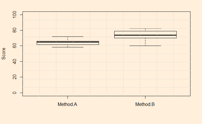
As done before, we plot the data first; we use a box plot.

2-Sample t-test
The R code for the 2-sample t-test is the same (“t.test”) as before, but you need to input both sets of data in it.
AB_data <- data.frame(Method.A = c(60.12, 65.7, 70.1, 62.14, 71.8, 62.1, 64.9, 64.8, 59.1, 65.9, 66.8, 61.5, 58.2, 61.8, 65.9), Method.B = c(70.62, 73.7, 82.1, 72.14, 77.1, 63.1, 80.4, 61.3, 60.1, 75.8, 78.5, 69.9, 70, 82.1, 79.1))

t.test(AB_data$Method.A, AB_data$Method.B, var.equal = TRUE)
Two Sample t-test
data: AB_data$Method.A and AB_data$Method.B
t = -4.2402, df = 28, p-value = 0.00022
alternative hypothesis: true difference in means is not equal to 0
95 percent confidence interval:
-13.357755 -4.655578
sample estimates:
mean of x mean of y
64.05733 73.06400 Before jumping to the answers, you may have noticed that I have used var.equal = TRUE here. In other words, I have assumed the variances of each group to be equal; well, more or less similar! Depending on the variances, there are two methods: the standard method is used when the variances are similar. When they are different, we need to use the Welch t-test. Let’s check the standard deviations of the groups. They are 3.86 and 7.27.
We’ll make no assumptions here, and I repeat the calculations using var.equal = FALSE. Here are the results.
t.test(AB_data$Method.A, AB_data$Method.B, var.equal = FALSE)
	Welch Two Sample t-test

data:  AB_data$Method.A and AB_data$Method.B
t = -4.2402, df = 21.308, p-value = 0.0003561
alternative hypothesis: true difference in means is not equal to 0
95 percent confidence interval:
 -13.42015  -4.59318
sample estimates:
mean of x mean of y
 64.05733  73.06400
Similar answers suggest that variances are, indeed, close to each other.
Interpreting results
We will start with the p-value now. p = 0.0003561, which is less than the standard significance level of 0.05. Therefore, we can reject the null hypothesis. i.e., the sample data suggest that the population means are different.
The 90% confidence interval [-13.4, -4.6] escapes zero, which is no more a surprise and reinforces the fact that the null hypothesis, zero difference between the means, is not valid here. The negative sign on the difference only means that the mean of method A is lower than method B.

