We have created the background on the Shark attack problem to explain how Bayesian inference operates for updating knowledge of an event, in this case, a rare one. Let’s have a quick recap first. We chose Poisson distribution to describe the likelihood (the chances of that data on attacks, given a particular set of occurrences) because we knew these were rare and uncorrelated events. And the Gamma for describing the prior probability of occurrences as it can give a continuous set of instances ranging from zero to infinity.
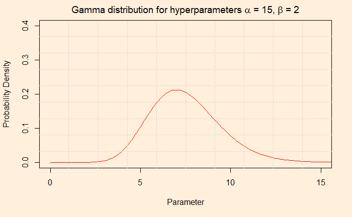
And if you like to know how those two functions work, see the following two plots.
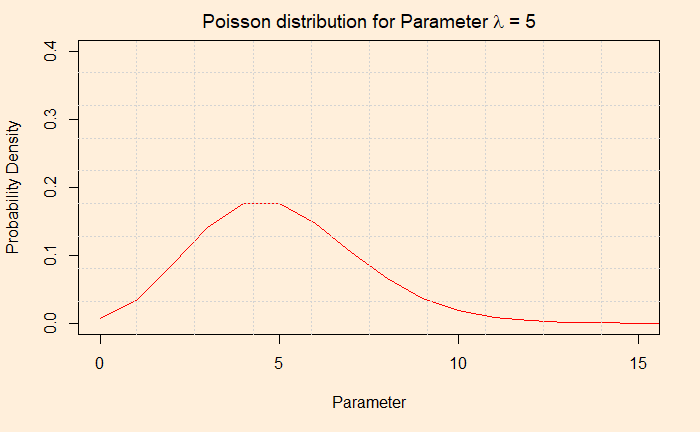
The first plot gives the probability of one occurrence, two occurrences, 3, 4, 5, 6 …, when the mean occurrence is five. The value the X-axis take is discrete: you can not have the probability of 1.8 episodes of a shark attack!
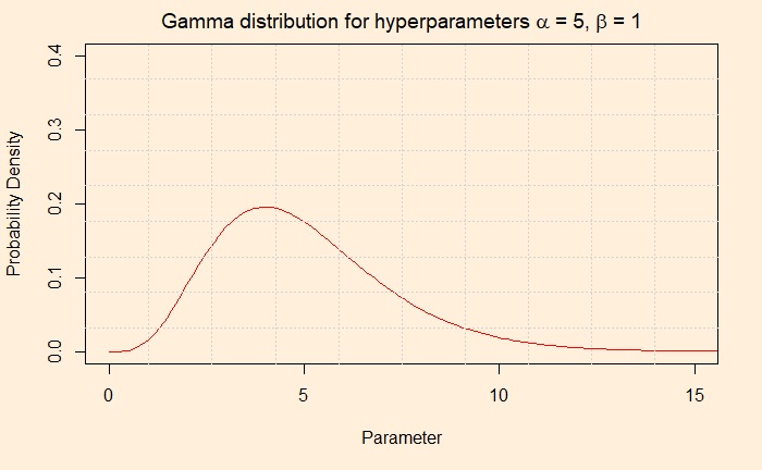
The second plot provides the probability of the parameter (occurrence or episode) through the gamma pdf using those two hyperparameters, alpha and beta.
Bayesian Inference
The form of Bayes’ theorem now becomes.
![]()
Then the magic happens, and the complicated looking equation solves into a Gamma distribution function. You will now realise the choice of Gamma as the prior was not an accident, but it was because of its conjugacy with the Poisson. But we have seen that before.
The Posterior
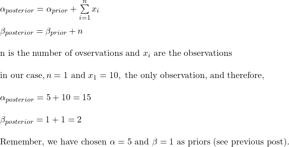
The posterior is a Gamma pdf with the following hyperparameters.
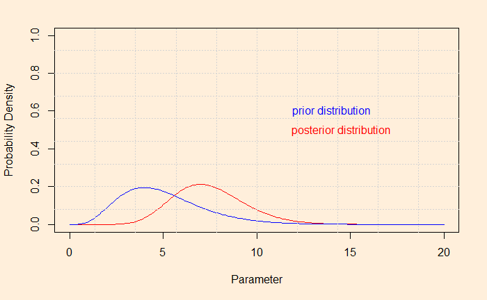
And, if you want to see the shift of the hypothesis from prior to posterior after the evidence,
