Let’s demonstrate the analysis using an example. An advertising campaign for a product surveyed 16 people, and 6 of them responded positively. What are the expected product sales when it is launched on a large scale?
The simplest way is to divide 6 by 16 = 38% and conclude that this is the potential hit rate. However, this has large uncertainty (due to the small sample size), and we must account for that. Remember the steps of Bayesian inference.
- Data
- A generative model: a mathematical formulation that can give simulated data from the input of parameters.
- Priors: information for the model before seeing the data
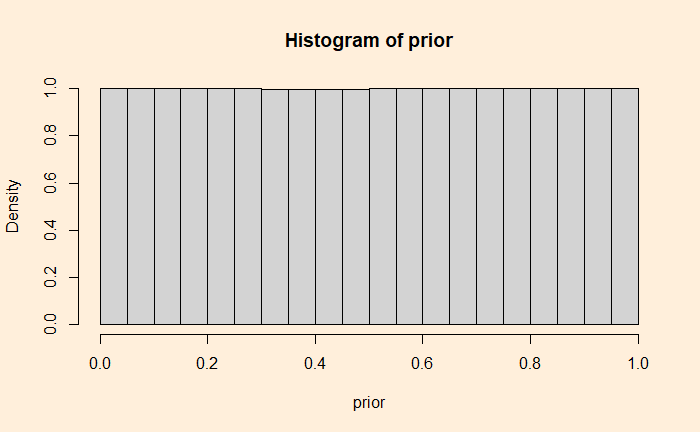
We have data, and we need a generative model. The aim is to determine what parameter would have generated this data, i.e., the likely rate of positive ‘vibe’ in public that would have resulted in 6 out of 16. Assuming individual preferences are independent, we can utilise the binomial probability distribution as the generative model. Now, we need the parameter value. Since we don’t know that, we use all possible values or a uniform distribution.

Now, we start fitting the model. Draw a random parameter value from the prior.
prior <- runif(1, 0, 1)0.4751427Run the model using 0.4751427
rbinom(1, size = 16, prob = 0.4751427)8Well, this doesn’t fit because the output is not 6, but 8. Repeat this sampling and model-runs several times, collect the parameter values that result in 6 and make a histogram.

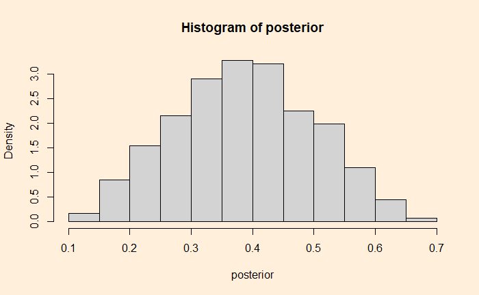
The first takeaway is that parameter values below 0.1 and above 0.7 have rarely resulted in the observed data. The median posterior turns out to be 0.386.

Finding the posterior distribution is the goal of Bayesian analysis. The value 0.386 (38.6%) is the most probable parameter value that would have resulted in the observed data—the famous “maximum likelihood estimate.”
Reference
Introduction to Bayesian data analysis – part 1: What is Bayes?: rasmusab

