Linear Programming in R

A factory makes two products, Alpha and Beta, using four ingredients: A, B, C and D. The quantity requirement for each component per kg of the product is:

	A	B	C	D
Alpha	500	750	150	200
Beta	500	625	100	300

The profits from the products (per kg) are

	Profit
Alpha	45
Beta	50

The maximum daily demands for the product (kg) are:

	Profit
Alpha	50
Beta	20

If there are constraints (as below) on the supply of the ingredients, what should be the product mix?

A	B	C	D
20000	42000	10400	9600

Linear Programming

This is an example of the application of linear programming (LP), a popular tool in prescriptive analysis. The solution starts by identifying the decision variables and the objective function.

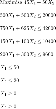
The quantities of the two products are the decision variables. Let’s name them X1 (alpha) and X2 (beta). The objective (function) is to maximise the profit, 45 X1 + 50 X2. All the other information provided above are constraints (on the ingredients, demand, etc). The LP formulation is given below:

$\\ \textrm{Maximise } 45 X_1 + 50 X_2 \\ \\ 500 X_1 + 500 X_2 \le 20000 \\ \\ 750 X_1 + 625 X_2 \le 42000 \\ \\ 150 X_1 + 100 X_2 \le 10400 \\ \\ 200 X_1 + 300 X_2 \le 9600 \\ \\ X_1 \le 50 \\ \\ X_2 \le 20 \\ \\ X_1 \ge 0 \\ \\ X_2 \ge 0$

We use R to solve the set of equations. The package used is ‘lpSolve’.

library(lpSolve)
f.obj <- c(45, 50)
f.con <- matrix (c(500, 500, 750, 625, 150, 100, 200, 300, 1, 0, 0, 1), nrow = 6, byrow = TRUE)
f.dir <- c("<=", "<=")
f.rhs <- c(20000, 42000, 10400, 9600, 50, 30)

results <- lp ("max", f.obj, f.con, f.dir, f.rhs)
results
results$solution

Success: the objective function is 1880 
24 16

The maximum profit is 1880, and the optimal production quantities are alpha = 24 and beta = 16.

Linear Programming

Related Posts