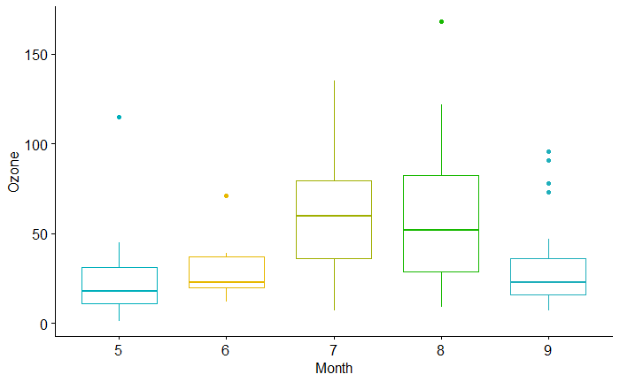
Here are five months of quality data on Ozone concentration. The task is to test if one month’s data is significantly different from any other month’s.
The first thing to graph the monthly variations of ozone in summary plots: a boxplot is one good choice.

library(ggpubr)
data("airquality")
AQ_data <- airquality
ggboxplot(AQ_data, x = "Month", y = "Ozone",
          color = "Month", palette = c("#00AFBB", "#E7B800", "#a0AF00", "#17B800", "#20AFBB"),
        ylab = "Ozone", xlab = "Month") +
theme(legend.position="none")
Getting quantitative
Let’s do a hypothesis test. A few quick Shapiro tests suggest only month 7 followed a normal distribution. So, we will use a non-parametric test. The Kruskal–Wallis test is one of them.
kruskal.test(Ozone ~ Month, data = airquality) Kruskal-Wallis rank sum test
data: Ozone by Month
Kruskal-Wallis chi-squared = 29.267, df = 4, p-value = 6.901e-06Yes, monthly behaviours are not similar. If you want pair-wise testing, we can use a pair-wise Wilcoxon rank-sum test.
pairwise.wilcox.test(AQ_data$Ozone, AQ_data$Month) Pairwise comparisons using Wilcoxon rank sum test with continuity correction
data: AQ_data$Ozone and AQ_data$Month
5 6 7 8
6 0.5775 - - -
7 0.0003 0.0848 - -
8 0.0011 0.1295 1.0000 -
9 0.4744 1.0000 0.0060 0.0227
P value adjustment method: holm The conclusion: Significant differences are seen:
Month 5 vs Month 7 and Month 8
Month 9 vs Month 7 and Month 8

