Confusion Matrix and Statistics

          Reference
Prediction Female Male
    Female     55   24
    Male       64  383

               Accuracy : 0.8327
                 95% CI : (0.798, 0.8636)
    No Information Rate : 0.7738
    P-Value [Acc > NIR] : 0.0005217

                  Kappa : 0.4576

 Mcnemar's Test P-Value : 3.219e-05

            Sensitivity : 0.4622
            Specificity : 0.9410
         Pos Pred Value : 0.6962
         Neg Pred Value : 0.8568
             Prevalence : 0.2262
         Detection Rate : 0.1046
   Detection Prevalence : 0.1502
      Balanced Accuracy : 0.7016

       'Positive' Class : Female
We see the prediction we did had high overall accuracy. At the same time, we see it had a low sensitivity. It happened because of the low prevalence (proportion of females), 23%. That means failing to call actual females as females (low sensitivity) does not lower the accuracy as much as it would have by incorrectly calling males as females.
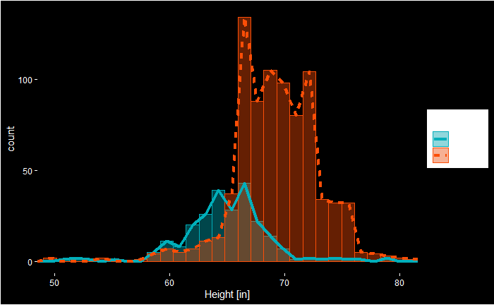
Here is the R code behind this fancy plot!
heights %>%
  ggplot(aes(x = height)) +
geom_histogram(aes(color = sex, fill = sex), alpha = 0.4, position = "identity") +
  geom_freqpoly( aes(color = sex, linetype = sex), bins = 30, size = 1.5) +
    scale_fill_manual(values = c("#00AFBB", "#FC4E07")) +
  scale_color_manual(values = c("#00AFBB", "#FC4E07")) +
  coord_cartesian(xlim = c(50, 80)) +
  scale_x_continuous(breaks = seq(50, 80, 10), name = "Height [in]") +
  theme(text = element_text(color = "white"),
        panel.background = element_rect(fill = "black"),
        plot.background = element_rect(fill = "black"),
        panel.grid = element_blank(),
        axis.text = element_text(color = "white"),
        axis.ticks = element_line(color = "white"))
Looking at the plot, we see that the cut-off we used, 64 inches, misses a significant proportion of females. Let’s re-run the simulations after adding two more points (66 inches) to the cut-off.
Confusion Matrix and Statistics

          Reference
Prediction Female Male
    Female     82   66
    Male       33  345

               Accuracy : 0.8118
                 95% CI : (0.7757, 0.8443)
    No Information Rate : 0.7814
    P-Value [Acc > NIR] : 0.049151

                  Kappa : 0.5007

 Mcnemar's Test P-Value : 0.001299

            Sensitivity : 0.7130
            Specificity : 0.8394
         Pos Pred Value : 0.5541
         Neg Pred Value : 0.9127
             Prevalence : 0.2186
         Detection Rate : 0.1559
   Detection Prevalence : 0.2814
      Balanced Accuracy : 0.7762

'Positive' Class : Female 
