Does aiming high get you the goal?

Let’s recap the penalty data that we discussed last time.

	Attempt	Success	goal %
Total	279	195	69.9%
Top section	63	46	73.0%
Middle section	87	63	72.4%
Bottom section	129	86	66.7%

Is top really on top?

We start with the null hypothesis, H₀:
H₀ = Success rate at the section of the post is no different from the average rate of 0.699

There are many ways to test this hypothesis. The simplest way is to use the ‘prop.test’ in R. Note that we use a 90% confidence interval, which gives a better chance to disprove the premise.

prop.test(x = sum(top_suc), n = sum(top_suc) + sum(top_fai), p = 0.6989247, correct = FALSE, conf.level = 0.9)

1-sample proportions test without continuity correction

data:  sum(top_suc) out of sum(top_suc) + sum(top_fai), null probability 0.6989247
X-squared = 0.29207, df = 1, p-value = 0.5889
alternative hypothesis: true p is not equal to 0.6989247
90 percent confidence interval:
 0.6301125 0.8112506
sample estimates:
        p 
0.7301587 

The p-value of 0.5889 suggests the hypothesis stays; there is no evidence to suggest that the top brings any advantage! The global average success rate (0.699) is well within the 90% confidence interval [0.63,0.81] of 46 in 63.

Penalty as a binomial trial

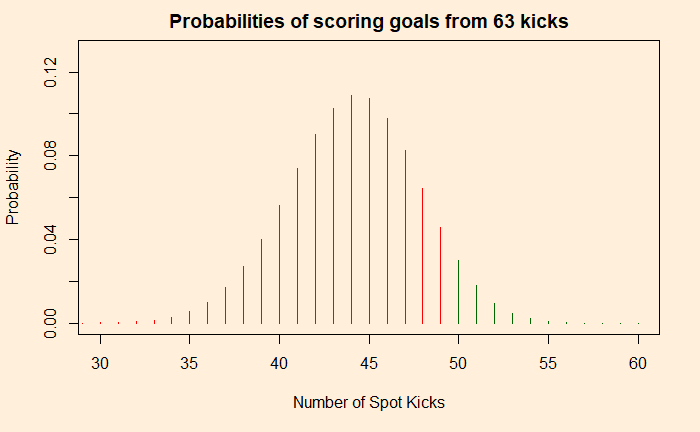
Another way to understand this problem is to consider penalty kicks as a binomial trial (with the probability of success = 0.699). If you kick 63 balls to the top section of the post, the expected number of goals, under the assumption of no special advantage, is between 38 and 50.

conf_int <- 0.9
qbinom(c((1-(1-conf_int)/2), (1-conf_int)/2), size = 63, prob = 0.7)

You can see that scoring 46 goals is well within limits.