Bayesian inference is a statistical technique to update the probability of a hypothesis using available data with the help of Bayes’ theorem. A long and complicated sentence! We will try to simplify this using an example – finding the bias of a coin.
Let’s first define a few terms. The bias of a coin is the chance of getting the required outcome; in our case, it’s the head. Therefore, for a fair coin, the bias = 0.5. So the objective of experiments is to toss coins and collect the outcomes (denoted by gamma). For simplicity, we give one for every head and zero for every tail.
![]()
The next term is the parameter (theta). While the outcomes are only two – head or tail, their tendency to appear can reside on a range of parameters between zero and 1. As we have seen before, theta = 0.5 represents the state of the unbiased coin.
The objective of Bayesian inference is to estimate the parameter or the density distribution of the parameters using data and starting guesses. For example:

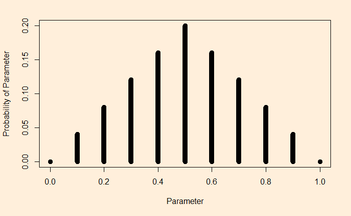
In this picture, you can see an assumed probability distribution of coins made from a factory. In a way, this is to say that the factory produces ranges of coins; we think the highest probability to be theta = 0.5, the perfect unbiased coin, although all sorts of other imperfections are possible (theta < 0.5 for tail-biased and theta > 0.5 for head-biased).
The model
It is the mathematical expression for the likelihood function for every possible parameter. For coin tosses, we know we can use the Bernoulli distribution.
![]()
If you toss a number of coins, the probability of the set of outcomes becomes:

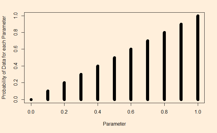
Suppose we flip a coin and get heads. We substitute gamma = 1 for each of the theta values. A plot of this function for the following type appears:

Let’s spend some time understanding this plot. The plot says: if I have a theta = 1, that is a 100% head-biased coin, the likelihood of getting a head on a coin flip is 1. If it is 0.9, then 0.9 etc., until you reach a tail-biased one at theta = 0.
Imagine, I did two flips and got a head and a tail:

The interpretation is straightforward. To take the extreme left point: If it was a tail-biased coin (the parameter, theta = 0), the probability of getting one head and one tail is extremely low. Same for the extreme right (the head-biased).
Posterior from prior and likelihood
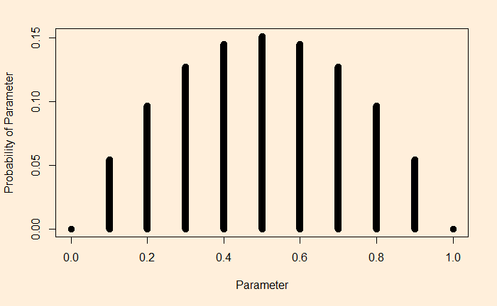
We have prior assumptions and the data. We are ready to use Bayes’ rule to get the posterior.

