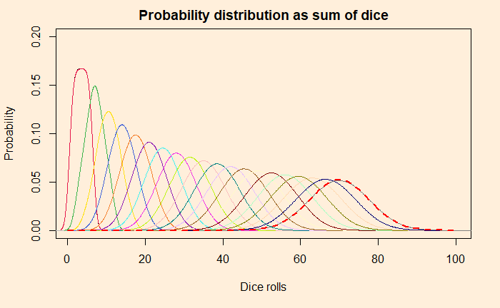
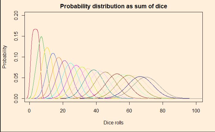
We have seen how outcomes from games with uniform probabilities add up to a normal distribution. Today we make a little R program that simulates this and plots the probability densities on one graph. In the end, we will explore how to construct the normal distribution that it approximates. Here is the plot that shows the rolling of up to 20 dice, starting from a single one.
Simulating the dice
As usual, we use the sample() function to throw out random outcomes by providing six options with equal probabilities. The sampling is then placed inside a loop that keeps on adding outputs.
plots <- 20
sides <- 6
   roll_ini <- replicate(100,0)
   roll <- sample(seq(1:sides), 1000000, replace = TRUE, prob = replicate(sides,1/sides))
   Dist_ini <- density(roll, bw=0.9)

   par(bg = "antiquewhite1")
   plot(Dist_ini, ylim=c(0,0.2), xlim=c(1,100), main="Probability distribution as sum of dice", xlab = "Dice rolls", ylab =  "Probability")

 for (i in 1:plots){
   roll <- roll_ini + sample(seq(1:sides), 1000000, replace = TRUE, prob = replicate(sides,1/sides))
   Dist <- density(roll, bw=0.9)
   mycolors <- c('#e6194b', '#3cb44b', '#ffe119', '#4363d8', '#f58231', '#911eb4', '#46f0f0', '#f032e6', '#bcf60c', '#fabebe',  '#008080', '#e6beff', '#9a6324', '#fffac8', '#800000', '#aaffc3', '#808000', '#ffd8b1', '#000075', '#808080', '#ffffff', '#000000')
   lines(Dist, col = mycolors[i])
   roll_ini <- roll
 }
We then derive the normal distribution that corresponds to the above. The mean and standard deviation of rolling a die are:
![\\ \text{ mean } = E[X] = \sum\limits_{i=1}^6 x_i p_i = x_1p_1 + x_2p_2 + x_3p_3 + x_4p_4 + x_5p_5 + x_6p_6 \\ \\ = 1 * \frac{1}{6} + 2 * \frac{1}{6} +3 * \frac{1}{6} +4 * \frac{1}{6} +5 * \frac{1}{6} +6 * \frac{1}{6} = \frac{21}{6} = \frac{7}{2} = 3.5\\\\ \text {for n rolls,} \\ \\ E[X_1 + X_2 + ... + X_n] = E[X_1] + E[X_2] + ... + E[X_n] \\ \\ E[X + X + ... + X] = E[nX] = nE[X] = 3.5*n \\ \\ \text{variance} = Var[X] = E[(X - \mu)^2] \\ \\ Var[X] = \sum\limits_{i=1}^6 \frac{1}{6} (i-\frac{7}{2})^2) = \frac{1}{6} [ (- \frac{5}{2})^2 + (- \frac{3}{2})^2 + (- \frac{1}{2})^2 + (\frac{1}{2})^2 + ( \frac{3}{2})^2 + ( \frac{5}{2})^2] \\ \\ Var[X] = \frac{35}{12} \\ \\ \text{standard deviation } = \sigma = \sqrt{(Var[X])} = \sqrt{\frac{35}{12}} \\ \\ \text {for n rolls,} \\ \\ Var[(X+Y)] = Var[X] + Var[Y] + Cov(X,Y) \\ \\ Var[(nX)] = n*Var[X] + 0 \text{ , } Cov(X,X) = 0\\ \\ Var[(nX)] = \frac{35}{12} n \\\\ \sigma = \sqrt{\frac{35}{12} n}](https://thoughtfulexaminations.com/wp-content/ql-cache/quicklatex.com-dae737128427a51955019607d5d1b795_l3.png "Rendered by QuickLaTeX.com")
Add the following line at the end, and you get the comparison for normal distribution for rolls of 20 dice summed over.
norm_die <- 20
lines(seq(0,100), dnorm(seq(0,100), mean = norm_die*(7/2), sd = sqrt(norm_die*(35/12))), col = "red",lty= 2, lwd=2)