We have seen the Iris dataset before. It consists of 150 samples, 50 each from three species of Iris (Iris Setosa, Iris Virginica and Iris Versicolor). Four features, the length and the width of the sepals and petals (in cm), are available in the set.

These parameters can then be used to make predictive models to distinguish the species from each other.

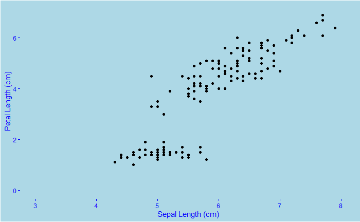
As we did before, we make a scatter plot between two features, Petal length versus Sepal length, followed by a 2D density plot.


You may already find Setosa is easily identifiable based on its short petal and sepal. In the last plot, we used the colour palette, ‘Spectral’.
library(tidyverse)
library(ggExtra)
plot <- iris %>% ggplot(aes(x = Sepal.Length, y=Petal.Length) ) +
geom_point(aes(colour = Species)) +
  stat_density_2d(aes(fill = ..density..), geom = "raster", contour = FALSE) +
  scale_fill_distiller(palette= "Spectral", direction=1) +

  xlim(3, 8) +
  ylim(0, 7) +
  xlab("Sepal Length (cm)") +
  ylab("Petal Length (cm)") +
  theme(text = element_text(color = "blue"),
        panel.background = element_rect(fill = "lightblue"),
        plot.background = element_rect(fill = "lightblue"),
        panel.grid = element_blank(),
        axis.text = element_text(color = "blue"),
        axis.ticks = element_line(color = "blue"))

ggMarginal(plot, type="density",groupColour = TRUE, groupFill = TRUE)
Let’s change the plot type at the margins from density to boxplot.

Another noticeable feature of Setosa is it has a wider sepal than the other two.


