1-Sample t-Test

We will do a 1-sample t-test from start to finish using R. You know about the t-test, and we have done it before.

What is a 1-sample t-test?

It is a statistical way of comparing the mean of a sample dataset with a reference value of the population. The reference value (reference mean) becomes the null hypothesis and what we do in the t-test is nothing but hypothesis testing.

Assumptions

There are a few key assumptions that we make before applying the test. First, it has to be a random sample. In other words, it has to be representative; otherwise, it would not provide any valid inference for the population. The second condition requires that the data must be continuous. Finally, the data should follow a normal distribution or have more than 20 observations.

Example

You have done a major revamp of the school curriculum this year. You know the state-level average test score last year was 50. You like to find out whether the average score this year is different from the previous. So, you conducted a random sample of 20 participants, and their scores are below:

Student	Score
1	40.5
2	50.1
3	60.2
4	51.3
5	42.1
6	57.2
7	37.9
8	47.2
9	58.3
10	60
11	61.2
12	52.5
13	66
14	55
15	58
16	55.1
17	47.4
18	52.1
19	63.1
20	52.1

Is that significant?

The mean = 53.365 suggests there was an improvement in students’ scores. But that is a quick conclusion; after all, we took only a sample, which will have variability, and, unlike the population mean, the sample means will follow a distribution. So we will do testing the following hypotheses:

The null hypothesis, N₀: The mean of the population this year is 50
The alternative hypothesis, N_A: The mean of the population this year is not 50
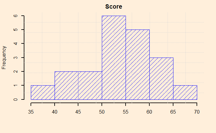
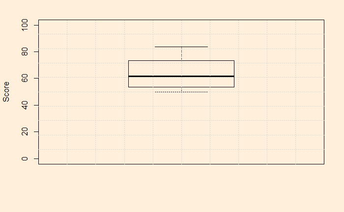
But, before that, let’s plot the data. It is a good habit that can already give a feel of the data quality, scatter, outliers etc.

The data look pretty ok, with no outliers, reasonably distributed etc. Now, the t-test. It’s simple: use the R function, t.test (stats package), and you get everything.

test_data <- data.frame(score = c(40.5,50.1,60.2, 51.3, 42.1, 57.2, 37.9, 47.2, 58.3, 60, 61.2, 52.5, 66, 55, 58, 55.1, 47.4, 52.1, 63.1, 52.1))
t.test(test_data$score, mu = 50)

The output is as follows

	One Sample t-test

data:  test_data$score
t = 1.9807, df = 19, p-value = 0.06229
alternative hypothesis: true mean is not equal to 50
95 percent confidence interval:
 49.80912 56.92088
sample estimates:
mean of x 
   53.365 

We shall see the inferences of this analysis in the next post.